Relative entropy and Kullback–Leibler divergence Dr. Konrad Völkel
Heinrich Heine University Düsseldorf
Logarithms ¶ The elementary properties of the logarithm – definition, change of base, bit and nat – are covered in the digression in the chapter Expected value and variance
Let l : { 1 , … } = N > 0 → R l \colon \{1,\dots\} = \mathbb{N}_{>0} \to \mathbb{R} l : { 1 , … } = N > 0 → R
l ( a b ) = l ( a ) + l ( b ) l(ab) = l(a) + l(b) l ( ab ) = l ( a ) + l ( b )
l ( n + 1 ) ≥ l ( n ) l(n+1) \geq l(n) l ( n + 1 ) ≥ l ( n ) c ∈ R c \in \mathbb{R} c ∈ R l ( n ) = c ln ( n ) l(n) = c \ln(n) l ( n ) = c ln ( n )
Equally clearly, the same lemma holds for log 2 \log_2 log 2 ln \ln ln
So if we want to count something in such a way that the count of a product is the sum of the individual counts, we have to use a logarithm.
We want to show that for functions f , g : N > 0 → R f,g \colon \mathbb{N}_{>0} \to \mathbb{R} f , g : N > 0 → R
f ( n ) g ( 2 ) = f ( 2 ) g ( n ) f(n) g(2) = f(2) g(n) f ( n ) g ( 2 ) = f ( 2 ) g ( n ) always holds, since with g = ln g = \ln g = ln c = f ( 2 ) c=f(2) c = f ( 2 )
Let n , k , m ∈ N n,k,m \in \mathbb{N} n , k , m ∈ N 2 m − 1 ≤ n k ≤ 2 m 2^{m-1} \leq n^k \leq 2^m 2 m − 1 ≤ n k ≤ 2 m
f ( 2 m − 1 ) ≤ f ( n k ) ≤ f ( 2 m ) f(2^{m-1}) \leq f(n^k) \leq f(2^m) f ( 2 m − 1 ) ≤ f ( n k ) ≤ f ( 2 m ) and additivity gives
( m − 1 ) f ( 2 ) ≤ k f ( n ) ≤ m f ( 2 ) (m-1)f(2) \leq kf(n) \leq mf(2) ( m − 1 ) f ( 2 ) ≤ k f ( n ) ≤ m f ( 2 ) The same chain of inequalities holds for g g g f f f
− m g ( 2 ) ≤ − k g ( n ) ≤ − ( m − 1 ) g ( 2 ) . -mg(2) \leq -kg(n) \leq -(m-1)g(2). − m g ( 2 ) ≤ − k g ( n ) ≤ − ( m − 1 ) g ( 2 ) . Adding the two chains of inequalities and simplifying gives
− f ( 2 ) g ( 2 ) ≤ k ( f ( n ) g ( 2 ) − f ( 2 ) g ( n ) ) ≤ f ( 2 ) g ( 2 ) -f(2)g(2) \leq k\left(f(n)g(2) - f(2)g(n)\right) \leq f(2)g(2) − f ( 2 ) g ( 2 ) ≤ k ( f ( n ) g ( 2 ) − f ( 2 ) g ( n ) ) ≤ f ( 2 ) g ( 2 ) Dividing by k k k k → ∞ k \to \infty k → ∞ f ( n ) g ( 2 ) − f ( 2 ) g ( n ) → 0 f(n)g(2) - f(2)g(n) \to 0 f ( n ) g ( 2 ) − f ( 2 ) g ( n ) → 0 k → ∞ k \to \infty k → ∞
If a continuous function F : R → R F \colon \mathbb{R} \to \mathbb{R} F : R → R F ( x y ) = x F ( y ) + F ( x ) y F(xy) = xF(y) + F(x)y F ( x y ) = x F ( y ) + F ( x ) y F ( x ) / x F(x)/x F ( x ) / x c ∈ R c \in \mathbb{R} c ∈ R F ( x ) = − x log ( x ) c F(x) = -x\log(x)c F ( x ) = − x log ( x ) c
The function g ( x ) : = F ( x ) / x g(x) := F(x)/x g ( x ) := F ( x ) / x g ( x y ) = g ( x ) + g ( y ) g(xy) = g(x) + g(y) g ( x y ) = g ( x ) + g ( y ) c ′ c' c ′ g ( x ) = c ′ log ( x ) g(x) = c'\log(x) g ( x ) = c ′ log ( x ) c : = − c ′ c:=-c' c := − c ′
The logarithm is a concave function, that is, for a convex combination λ x + μ y \lambda x + \mu y λ x + μ y λ + μ = 1 \lambda + \mu = 1 λ + μ = 1 0 ≤ λ , μ ≤ 1 0 \leq \lambda, \mu \leq 1 0 ≤ λ , μ ≤ 1
λ log ( x ) + μ log ( y ) ≤ log ( λ x + μ y ) \lambda \log(x) + \mu \log(y) \leq \log(\lambda x + \mu y) λ log ( x ) + μ log ( y ) ≤ log ( λ x + μ y ) Idea:
The derivative of log ( x ) \log(x) log ( x ) 1 x \frac{1}{x} x 1 ( 0 , ∞ ) (0,\infty) ( 0 , ∞ ) log ( x ) \log(x) log ( x ) < < < ≤ \leq ≤
We have argued this heuristically before; now we can prove it rigorously:
If p = ( p 1 , … , p n ) p = (p_1,\dots,p_n) p = ( p 1 , … , p n ) Ω = { 1 , … , n } \Omega = \{1,\dots,n\} Ω = { 1 , … , n } H ( p ) ≤ log ( n ) H(p) \leq \log(n) H ( p ) ≤ log ( n )
We use the fact that the sum in the definition of the entropy is a convex combination, and that the logarithm is concave:
H ( p ) = ∑ i = 1 , p i ≠ 0 n p i log 1 p i H(p) = \sum_{i=1, p_i\neq 0}^n p_i \log \frac{1}{p_i} H ( p ) = ∑ i = 1 , p i = 0 n p i log p i 1
≤ log ( ∑ i = 1 , p i ≠ 0 n p i 1 p i ) \leq \log \left( \sum_{i=1, p_i\neq 0}^n p_i \frac{1}{p_i} \right) ≤ log ( ∑ i = 1 , p i = 0 n p i p i 1 )
≤ log ( ∑ i = 1 n 1 ) = log ( n ) \leq \log\left( \sum_{i=1}^n 1 \right) = \log(n) ≤ log ( ∑ i = 1 n 1 ) = log ( n )
Definition and properties ¶ Let p , r ∈ Δ n p,r \in \Delta_n p , r ∈ Δ n R n \mathbb{R}^n R n entropy (also: Kullback–Leibler divergence D K L D_{KL} D K L p p p r r r
H ( p ∥ r ) : = ∑ i , p i > 0 n p i log ( p i r i ) ∈ R ∪ { ∞ } . H(p \Vert r) := \sum_{i,\ p_i > 0}^n p_i \log \left( \frac{p_i}{r_i} \right) \in \mathbb{R} \cup \{\infty\}. H ( p ∥ r ) := ∑ i , p i > 0 n p i log ( r i p i ) ∈ R ∪ { ∞ } .
Write u n = ( 1 n , … , 1 n ) ∈ Δ n u_n = (\frac{1}{n}, \dots, \frac{1}{n}) \in \Delta_n u n = ( n 1 , … , n 1 ) ∈ Δ n { 1 , … , n } \{1,\dots,n\} { 1 , … , n }
H ( p ∥ u n ) = H ( u n ) − H ( p ) = log ( n ) − H ( p ) H(p \Vert u_n) = H(u_n) - H(p) = \log(n) - H(p) H ( p ∥ u n ) = H ( u n ) − H ( p ) = log ( n ) − H ( p ) H ( p ∥ r ) = 0 if and only if p = r H(p \Vert r) = 0 \text{ if and only if } p=r H ( p ∥ r ) = 0 if and only if p = r (without proof)
H ( p ∥ r ) ≥ 0 H(p \Vert r) \geq 0 H ( p ∥ r ) ≥ 0 H ( p ∥ r ) = ∑ p i log ( p i r i ) = − ∑ p i log ( r i p i ) H(p \Vert r) = \sum p_i \log \left( \dfrac{p_i}{r_i} \right) = -\sum p_i \log \left( \dfrac{r_i}{p_i} \right) H ( p ∥ r ) = ∑ p i log ( r i p i ) = − ∑ p i log ( p i r i ) log ( a / b ) = − log ( b / a ) \log(a/b) = -\log(b/a) log ( a / b ) = − log ( b / a ) ≥ − log ( ∑ p i r i p i ) ≥ − log ( ∑ r i ) = − log 1 = 0 \geq - \log \left( \sum p_i \dfrac{r_i}{p_i} \right) \geq - \log \left( \sum r_i \right) = -\log 1 = 0 ≥ − log ( ∑ p i p i r i ) ≥ − log ( ∑ r i ) = − log 1 = 0
where we have again used the concavity of the logarithm.
Relative entropy is not symmetric, and it can become infinite. Let p t : = ( t , 1 − t ) p_t := (t,\ 1-t) p t := ( t , 1 − t ) 0 < t < 1 0 < t < 1 0 < t < 1 t t t
H ( u 2 ∥ p t ) = 1 2 log 1 2 t + 1 2 log 1 2 ( 1 − t ) → t → 0 ∞ , H\left(u_2 \,\Vert\, p_t\right) = \frac{1}{2} \log \frac{1}{2t} + \frac{1}{2}\log \frac{1}{2(1-t)} \xrightarrow{t \to 0} \infty, H ( u 2 ∥ p t ) = 2 1 log 2 t 1 + 2 1 log 2 ( 1 − t ) 1 t → 0 ∞ , since the first summand grows without bound, like − 1 2 log t -\frac12\log t − 2 1 log t
H ( p t ∥ u 2 ) = log ( 2 ) − H ( p t ) , H ( p t ) = − t log t − ( 1 − t ) log ( 1 − t ) → t → 0 0 , H\left(p_t \,\Vert\, u_2\right) = \log(2) - H(p_t), \qquad H(p_t) = -t\log t - (1-t)\log(1-t) \xrightarrow{t \to 0} 0, H ( p t ∥ u 2 ) = log ( 2 ) − H ( p t ) , H ( p t ) = − t log t − ( 1 − t ) log ( 1 − t ) t → 0 0 , so H ( p t ∥ u 2 ) → log 2 H(p_t \Vert u_2) \to \log 2 H ( p t ∥ u 2 ) → log 2 p t p_t p t p t p_t p t
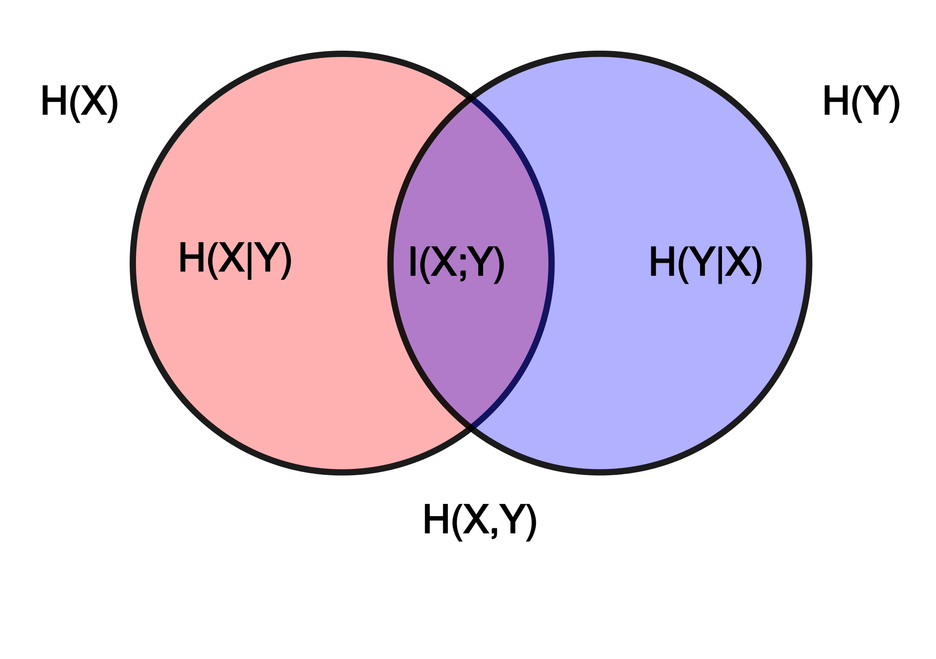
Joint entropy ¶ H ( X ) + H ( Y ) ≥ H ( X , Y ) ≥ max ( H ( X ) , H ( Y ) ) H(X) + H(Y) \geq H(X,Y) \geq \max\left( H(X), H(Y) \right) H ( X ) + H ( Y ) ≥ H ( X , Y ) ≥ max ( H ( X ) , H ( Y ) ) If X , Y X, Y X , Y H ( X , Y ) = H ( X ) + H ( Y ) H(X, Y) = H(X) + H(Y) H ( X , Y ) = H ( X ) + H ( Y )
The mutual information (also transinformation ) of two random variables X , Y X,Y X , Y
I ( X ; Y ) : = H ( X ) + H ( Y ) − H ( X , Y ) = H ( X , Y ∥ X × Y ) I(X;Y) := H(X)+H(Y)-H(X,Y)= H(X,Y \Vert X\times Y) I ( X ; Y ) := H ( X ) + H ( Y ) − H ( X , Y ) = H ( X , Y ∥ X × Y ) Here H ( ⋅ ∥ ⋅ ) H(\cdot \Vert \cdot) H ( ⋅ ∥ ⋅ ) distribution of ( X , Y ) (X,Y) ( X , Y ) P X × P Y P_X \times P_Y P X × P Y ( X , Y ) (X,Y) ( X , Y ) X X X Y Y Y
A very common application of mutual information is in clustering.
Suppose we have clustered a dataset by some method of our choice –
that is, arrived at an estimated class membership (say 1, 2 or 3 as a label) –
and a subset of the data has been classified by hand (for testing).
Then we can compute the mutual information of these two class variables to quantify how well the clustering worked on the test data.
The advantage is that the concrete labels no longer matter
(that is, the method is invariant under permutation of the class names).
The conditional entropy of X X X Y Y Y
H ( X ∣ Y ) : = H ( X ) − I ( X ; Y ) H(X|Y) := H(X) - I(X;Y) H ( X ∣ Y ) := H ( X ) − I ( X ; Y ) The mutual information of X X X I ( X ; X ) = H ( X ) I(X;X) = H(X) I ( X ; X ) = H ( X )
If X , Y X,Y X , Y I ( X ; Y ) = H ( X ) + H ( Y ) − ( H ( X ) + H ( Y ) ) = 0 I(X;Y) = H(X) + H(Y) - (H(X) + H(Y)) = 0 I ( X ; Y ) = H ( X ) + H ( Y ) − ( H ( X ) + H ( Y )) = 0
H ( X ∣ Y ) = H ( X , Y ) − H ( Y ) H(X|Y) = H(X,Y) - H(Y) H ( X ∣ Y ) = H ( X , Y ) − H ( Y ) and if X , Y X,Y X , Y H ( X ∣ Y ) = H ( X ) H(X|Y) = H(X) H ( X ∣ Y ) = H ( X )
Entropic Bayes’ theorem
H ( X ∣ Y ) = H ( Y ∣ X ) + H ( X ) − H ( Y ) H(X|Y) = H(Y|X) + H(X) - H(Y) H ( X ∣ Y ) = H ( Y ∣ X ) + H ( X ) − H ( Y ) If X X X Y Y Y Y Y Y X = f ( Y ) X = f(Y) X = f ( Y ) f = m o d 2 f = \mod 2 f = mod 2 H ( X , Y ) = H ( Y ) H(X,Y) = H(Y) H ( X , Y ) = H ( Y ) H ( X ∣ Y ) = 0 H(X|Y) = 0 H ( X ∣ Y ) = 0
Figure 1: Entropy, conditional entropy, joint entropy and mutual information in a Venn diagram. Figure: Wikimedia Commons, user KonradVoelkel
A summand with p i > 0 p_i > 0 p i > 0 r i = 0 r_i = 0 r i = 0 ∞ \infty ∞ log 0 = − ∞ \log 0 = -\infty log 0 = − ∞ r r r p p p
Careful : some authors unfortunately write the cross-entropy as H ( X , Y ) H(X, Y) H ( X , Y ) H ( X ; Y ) H(X;Y) H ( X ; Y ) I ( X ; Y ) I(X;Y) I ( X ; Y )
H ( X ; Y ) = H ( X ) + H ( X ∥ Y ) H(X; Y) = H(X) + H(X \Vert Y) H ( X ; Y ) = H ( X ) + H ( X ∥ Y ) If we hold X X X Y Y Y H ( X ; Y ) H(X;Y) H ( X ; Y ) H ( X ∥ Y ) H(X \Vert Y) H ( X ∥ Y )
In deep learning you meet this observation under three names: negative log-likelihood , cross-entropy and KL divergence to the labels all refer to the same loss function for classification problems. The last two differ only by the constant H ( X ) H(X) H ( X ) Introduction to Deep Learning takes this connection for granted.
Otherwise, the cross-entropy is used considerably less often in the theory than the relative entropy (usually called the Kullback–Leibler divergence D K L D_{KL} D K L
Continuous entropy ¶ This section is not part of the course proper; it reaches ahead to measure theory (Radon–Nikodym derivative, invariant measures), which this course does not cover. On a first reading it is enough to take away the core statement: in the continuous case, entropy is only meaningfully defined relative to a reference measure, so relative entropy is the fundamental notion.
One might think that the formula H ( p ) = − ∑ p i log p i H(p) = -\sum p_i \log p_i H ( p ) = − ∑ p i log p i H ( P ) = − ∫ log P d P H(P) = -\int \log P dP H ( P ) = − ∫ log P d P
Let P P P f f f Ω ⊆ R n \Omega \subseteq \mathbb{R}^n Ω ⊆ R n
h ( X ) : = E ( − log ( f ( X ) ) ) = − ∫ Ω f ( x ) log f ( x ) d x h(X) := \mathbb{E}\left( -\log(f(X)) \right) = - \int_\Omega f(x) \log f(x) dx h ( X ) := E ( − log ( f ( X )) ) = − ∫ Ω f ( x ) log f ( x ) d x is called the differential entropy of X X X
It already has some of the pleasant properties we would expect of a continuous entropy, translation invariance for instance: h ( X ) = h ( X − v ) h(X) = h(X - v) h ( X ) = h ( X − v ) v ∈ R n v \in \mathbb{R}^n v ∈ R n
Unfortunately the differential entropy is not invariant under arbitrary transformations, not even under isomorphisms.
Jaynes suggested picturing ever finer histograms, that is, a set of N N N { x i } \{x_i\} { x i } M ( a , b ) = lim N → ∞ 1 N ( number of x i : a < x i < b ) M(a,b) = \lim_{N \to \infty} \frac{1}{N} (\text{number of } x_i : a < x_i < b) M ( a , b ) = lim N → ∞ N 1 ( number of x i : a < x i < b ) m m m M ( a , b ) = ∫ a b m ( x ) d x M(a,b) = \int_a^b m(x) dx M ( a , b ) = ∫ a b m ( x ) d x invariant measure .
With that in hand we write
lim N → ∞ log ( N ) − ∫ p ( x ) log p ( x ) m ( x ) d x \lim_{N \to \infty} \log(N) - \int p(x) \log \dfrac{p(x)}{m(x)} dx N → ∞ lim log ( N ) − ∫ p ( x ) log m ( x ) p ( x ) d x but since lim N → ∞ log ( N ) = ∞ \lim_{N \to \infty} \log(N) = \infty lim N → ∞ log ( N ) = ∞ h ( x ) h(x) h ( x )
H ( X ) : = − ∫ p ( x ) log p ( x ) m ( x ) d x H(X) := - \int p(x) \log \dfrac{p(x)}{m(x)} dx H ( X ) := − ∫ p ( x ) log m ( x ) p ( x ) d x The first thing to note is that the “discrete entropy” of a continuous distribution is really ∞ \infty ∞
A theoretical analysis of what h ( X ) h(X) h ( X ) H ( X ) H(X) H ( X ) H ( P , Q ) H(P,Q) H ( P , Q ) h ( X ) = − H ( f λ ∥ λ ) h(X) = -H(f\lambda \,\Vert\, \lambda) h ( X ) = − H ( f λ ∥ λ ) λ \lambda λ f f f X X X
Let P , R P,R P , R relative entropy H ( P ∥ R ) H(P \Vert R) H ( P ∥ R ) D K L ( P , R ) D_{KL}(P,R) D K L ( P , R )
H ( P ∥ R ) : = − ∫ Ω log ( d R d P ) d P H(P \Vert R) := - \int_\Omega \log \left( \dfrac{dR}{dP} \right) dP H ( P ∥ R ) := − ∫ Ω log ( d P d R ) d P where d R d P \dfrac{dR}{dP} d P d R
We will not pursue that any further either; instead we record that for P P P R R R p , r : R n → [ 0 , ∞ ) p,r \colon \mathbb{R}^n \to [0,\infty) p , r : R n → [ 0 , ∞ )
H ( P ∥ R ) = ∫ Ω p ( x ) log p ( x ) r ( x ) d x H(P \Vert R) = \int_\Omega p(x) \log \frac{p(x)}{r(x)} dx H ( P ∥ R ) = ∫ Ω p ( x ) log r ( x ) p ( x ) d x This expression, in turn, we may evaluate by Riemann sums (if the density functions are friendly enough).
If for instance n = 1 n=1 n = 1 Ω = R \Omega = \mathbb{R} Ω = R
H ( P ∥ R ) = ∫ R p ( x ) log p ( x ) r ( x ) d x H(P \Vert R) = \int_{\mathbb{R}} p(x) \log \dfrac{p(x)}{r(x)} dx H ( P ∥ R ) = ∫ R p ( x ) log r ( x ) p ( x ) d x = ∑ k = − ∞ ∞ ∫ k k + 1 p ( x ) log p ( x ) r ( x ) d x = \sum_{k = -\infty}^{\infty} \int_{k}^{k+1} p(x) \log \dfrac{p(x)}{r(x)}dx = ∑ k = − ∞ ∞ ∫ k k + 1 p ( x ) log r ( x ) p ( x ) d x
and bound each of the integrals on the right by a value, so as to estimate H ( P ∥ R ) H(P \Vert R) H ( P ∥ R )
H ( P ∥ R ) ≈ ∑ k = − ∞ ∞ p ( k ) log p ( k ) r ( k ) H(P \Vert R) \approx \sum_{k = -\infty}^{\infty} p(k) \log \dfrac{p(k)}{r(k)} H ( P ∥ R ) ≈ k = − ∞ ∑ ∞ p ( k ) log r ( k ) p ( k ) The subdivision into intervals of length 1 can of course be made as fine as we like, making the approximation as accurate as we like. Replacing a continuous distribution by such a discrete one is the analogue of forming a histogram.
If you still doubt that abstract information theory has any relevance to the practical work of data scientists and machine learning engineers, a trip into the Wikipedia page on applications of mutual information and conditional entropy is recommended.