Multivariate statistics: covariance and dependence - Data Science Lecture Notes from Konrad Völkel

Joint distribution and Bayes¶

More generally, $(X_1,X_3,X_9)$ is also called a marginal distribution of $X$ , as is any composition of $X$ with a linear projection $\pi \colon \mathbb{R}^n \to \mathbb{R}^m$ – not necessarily onto a coordinate (hyper)plane of the standard basis of $\mathbb{R}^n$ .

Remark

For a random variable $(X,Y) \colon \Omega \to \mathbb{R}^2$ ,

P((X,Y) = (x,y)) = P(X = x, Y=y) = P(Y = y | X = x)P(X = x)

(3)

by the definition of conditional probability.

In the pmf notation we also write

p(x,y) = p(y|x)p(x)

(4)

where this is to be read as a definition:

p(y|x) = \frac{p(x,y)}{p(x)}

(5)

More precisely, one writes the distributions with their random variables as subscripts when several are in play:

p_{X,Y}(x,y) = p_{Y|X}(y \mid x)\, p_X(x),

(6)

where, for each fixed $x$ with $p_X(x) > 0$ , the function $p_{Y|X}(\cdot \mid x)$ is the pmf of the conditional distribution of $Y$ (likewise in the continuous case, with densities instead of pmfs). This formula is called the product rule; the sum rule is the preceding remark – summing over the variable we are not interested in.

Statement 3 is the generalisation of $P(A \mid B) = P(A)$ from the chapter Expected value and variance: knowing $X$ does not shift the distribution of $Y$ . In the continuous case the same equivalence holds with densities, but only “almost everywhere” – densities, after all, are determined only up to null sets (see Continuous distributions).

Example

Why the base rate matters. A test detects a rare disease reliably: $99\,\%$ of those who have it are detected, and only $1\,\%$ of the healthy get a false positive. Even so, after a positive test the probability of actually having the disease is small. The reason is the base rate $P(A)$ : if only one person in a thousand is ill, then for every ill person correctly detected there are about ten healthy ones falsely flagged – the small error rate of $1\,\%$ is acting on a group a thousand times larger. In the language of the confusion matrix from the chapter Titanic EDA: the test is a classifier, the $99\,\%$ is its recall (its sensitivity), the $1\,\%$ its false positive rate, and what we are after is its precision – the proportion of ill people among those who test positive. With $A$ = “ill” and $B$ = “test positive”, Bayes’ theorem performs exactly this weighting:

P(A|B) = \dfrac{0.99 \cdot 0.001}{0.99 \cdot 0.001 + 0.01 \cdot 0.999} = \dfrac{0.00099}{0.00099 + 0.00999} \approx 0.09.

(8)

$P(A|B)$ is emphatically not $P(B|A)$ : it is $P(B|A)$ times the ratio $P(A)/P(B)$ , and $P(B)$ is dominated by the large group of the healthy. Confusing the two conditional probabilities is the base rate fallacy – common enough to have a name of its own. For the Titanic rule “women survive”, recall 0.68 and precision 0.74 were close together, because survivors and women are about equally frequent; here a base rate of one in a thousand stands between 0.99 and 0.09. (Where the denominator comes from is settled by the law of total probability below.)

To work out the denominator $P(B)$ , the following theorem often helps:

In Bayes’ theorem you can therefore replace the denominator by $P(B) = P(B|A)P(A) + P(B|A^c)P(A^c)$ when $A$ and its complement are all you have to go on.

We often apply this as follows: $Y$ is “known” and $X$ is the provisional model. We then call $Y=y$ the data $D$ and $X=x$ the hypothesis $H$ .

For data and hypothesis this gives

Example

How to work out a likelihood. So far $H$ and $D$ have been events with finitely many outcomes. In practice the hypothesis is usually a whole distribution. Suppose we have $n$ measurements $D = (x_1,\dots,x_n)$ and work with normal distributions: the hypothesis $H$ says that the data come from an $\mathcal{N}(\mu,\sigma^2)$ with $\mu = 0$ and $\sigma = 2$ . The likelihood $P(D \mid H)$ is then the probability (or probability density) of seeing exactly these $n$ values if the hypothesis is right – and since the measurements are taken to be independent, the joint density factorises into a product by the proposition above:

P(D \mid H) = \prod_{i=1}^n p_{\mu,\sigma}(x_i) = \prod_{i=1}^n \dfrac{1}{\sqrt{2\pi}\,\sigma} \exp\left( -\dfrac{(x_i - \mu)^2}{2\sigma^2} \right) \quad \text{with } \mu = 0,\ \sigma = 2.

(12)

Three roles have to be kept cleanly apart here: the data-generating distribution, which exists out in the world and which we do not know; the observed data $D$ , which we have; and the model distribution, which we declare to be our hypothesis. The likelihood compares the second with the third. If we let $\mu$ and $\sigma$ vary instead of holding them fixed, the number becomes a function $L(\mu,\sigma) := \prod_{i=1}^n p_{\mu,\sigma}(x_i)$ , and searching for the parameters that maximise it is the maximum likelihood principle – see Statistical models and estimators, where taking logarithms turns the product into a sum.

Example

Bayesian updating. Today’s posterior is tomorrow’s prior. In the disease-test example the probability of being ill after a positive test was about 0.09. If the test is repeated, independently of the first run, then 0.09 is now the prior $P(H)$ , the likelihood of a positive result is still 0.99 for the ill and 0.01 for the healthy, and the evidence is again worked out by total probability:

P(H|D) = \dfrac{0.99 \cdot 0.09}{0.99 \cdot 0.09 + 0.01 \cdot 0.91} \approx 0.91.

(14)

Two positive tests in a row turn one in a thousand first into nine per cent and then into ninety-one. Every new observation pushes the posterior further along, and the outcome depends on the initial prior: start at $P(H) = 0.001$ and you need two tests; start at 0.5 (because there are symptoms already, say) and a single test puts you at 0.99. This process is called Bayesian updating; the chapter Statistical models turns the likelihood into a general estimation procedure.

Covariance¶

First a warning familiar from the chapter Descriptive statistics: covariance and correlation measure a relationship across all the data points. If the data split into groups, the relationship within each group can have the opposite sign – see Simpson’s paradox. So the numbers in this chapter tell you something only once you know that the sample comes from a single population.

In particular, $\mathbb{V}(X) = \operatorname{Cov}(X,X)$ .

The covariance suffers from the same complaint as the variance: it depends on the scale. The cure is to normalise by the standard deviations:

Remark

For data. If $x, y \in \mathbb{R}^n$ are given as two columns of a table, you replace the expected value in the definitions by the mean and obtain the empirical covariance and the empirical correlation coefficient

\operatorname{Cov}(x,y) := \frac{1}{n} \sum_{i=1}^n (x_i - \bar x)(y_i - \bar y) = \frac{1}{n}\, \tilde x \cdot \tilde y, \qquad r := \frac{\operatorname{Cov}(x,y)}{\sigma(x)\,\sigma(y)} = \frac{\tilde x \cdot \tilde y}{\lVert \tilde x \rVert \, \lVert \tilde y \rVert},

(17)

with the centred vectors $\tilde x, \tilde y$ from the chapter Expected value and variance. The correlation coefficient of data is thus, quite literally, the cosine of the angle between the centred columns. It is the number np.corrcoef(x, y)[0, 1] prints in the chapter Titanic EDA; np.cov(x, y, ddof=0) gives the covariance matrix in the $n$ -version (without ddof=0, Numpy divides by $n-1$ here, unlike np.var). For the Iris exercise from the chapter Descriptive statistics you compute it once across all the rows and once per species:

x = datasets.load_iris().data; y = datasets.load_iris().target
print(np.corrcoef(x[:, 0], x[:, 1])[0, 1])                          # -0.118
for s in range(3):
    print(s, np.corrcoef(x[y == s, 0], x[y == s, 1])[0, 1])         # 0.743, 0.526, 0.457

Symmetry and bilinearity give us the rules of calculation that come up constantly in practice:

Proof

(1) $\mathbb{V}(X+Y) = \operatorname{Cov}(X+Y, X+Y) = \operatorname{Cov}(X,X) + \operatorname{Cov}(X,Y) + \operatorname{Cov}(Y,X) + \operatorname{Cov}(Y,Y)$ by bilinearity, and the two middle terms are equal by symmetry. (2) The constant random variable $\beta$ has expected value $\beta$ , so $\beta - \mathbb{E}\beta = 0$ and $\operatorname{Cov}(X,\beta) = \mathbb{E}((X - \mathbb{E}X) \cdot 0) = 0$ . (3) Bilinearity and (2): $\operatorname{Cov}(X+\beta, Y) = \operatorname{Cov}(X,Y) + \operatorname{Cov}(\beta, Y) = \operatorname{Cov}(X,Y)$ . (4) Multiply out the definition and use linearity of the expected value:

\mathbb{E}\big(XY - X\,\mathbb{E}Y - Y\,\mathbb{E}X + \mathbb{E}X\,\mathbb{E}Y\big) = \mathbb{E}(XY) - 2\,\mathbb{E}X\,\mathbb{E}Y + \mathbb{E}X\,\mathbb{E}Y = \mathbb{E}(XY) - \mathbb{E}X\,\mathbb{E}Y.

(18)

Rule (4) is the counterpart of the formula $\mathbb{V}(X) = \mathbb{E}(X^2) - (\mathbb{E}X)^2$ from the chapter Expected value and variance; for $X = Y$ the two coincide. From (1) it also follows that $\mathbb{V}(X_1 + \dots + X_n) = \sum_i \mathbb{V}(X_i)$ whenever the $X_i$ are pairwise uncorrelated.

Proof

In the discrete case, independence makes the joint pmf a product, $p(x,y) = p_X(x)\,p_Y(y)$ , and the double sum splits:

\mathbb{E}(XY) = \sum_{x}\sum_{y} x\,y\,p_X(x)\,p_Y(y) = \Big(\sum_x x\,p_X(x)\Big)\Big(\sum_y y\,p_Y(y)\Big) = \mathbb{E}(X)\,\mathbb{E}(Y).

(19)

In the continuous case the sums become integrals over the joint density $p(x,y) = p_X(x)\,p_Y(y)$ (joint densities are introduced in the next chapter), and the calculation is the same. Rule (4) then gives $\operatorname{Cov}(X,Y) = \mathbb{E}(XY) - \mathbb{E}X\,\mathbb{E}Y = 0$ .

The covariance therefore behaves like an inner product – but only “modulo constants”, since constant random variables have covariance 0 with everything, themselves included. This can be made rigorous by reading the covariance as an inner product on an $\mathcal{L}^2$ space of random variables in which two random variables differing only by a constant are identified. The correlation coefficient then plays the role of the cosine of the angle between two random variables. For data it literally is that (see the remark For data above); the “cosine similarity” so widespread in machine learning is the same cosine, just without the centring.

You can get some practice at “seeing” the correlation coefficient in a scatter plot of two variables, for instance with the game “Guess the Correlation” by Omar Wagih.

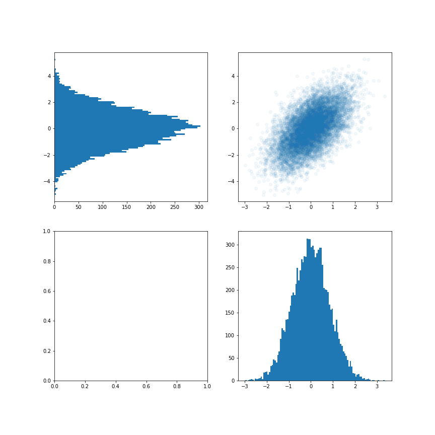
Figure 1:A sample from a bivariate normal distribution, with the two marginal histograms.

The picture shows why the correlation cannot be read off the individual variables. Each of the two marginal histograms is an unremarkable bell curve; they would look exactly the same if the correlation had the opposite sign, or were 0, because the marginal distributions do not depend on it. The relationship shows only in the joint scatter plot, in the tilt of the cloud of points. This is the observation made above about the joint distribution: it cannot be reconstructed from the individual ones.

What covariance and correlation mean geometrically we will see in the next chapter, on the multivariate normal distribution: there the covariance matrix describes the shape and position of the ellipses that are the contour lines of the density.