You have already met the basics of (discrete) probability theory in Mathematics for Computer Scientists 3. We will go over them again, as far as we need them. In this course we will mostly work with the probability mass function (for discrete random variables) and the probability density function (for continuous random variables), both of which build on the notion of a probability measure. At this point a short digression explains why things are done exactly this way, and how one might arrive at the notion of a probability measure in the first place. The notions of a sigma-algebra (-algebra) and of a measurable function are essential for proofs in probability theory, and for introducing more advanced notions (the ones mathematical finance or the theory of machine learning need) – here it is enough to take away when we are allowed to read past them.
Stochastics can be understood as an umbrella term for probability theory and statistics. Statistics builds probabilistic models from observations and draws conclusions from them. Probability theory investigates those models and the theory behind them.
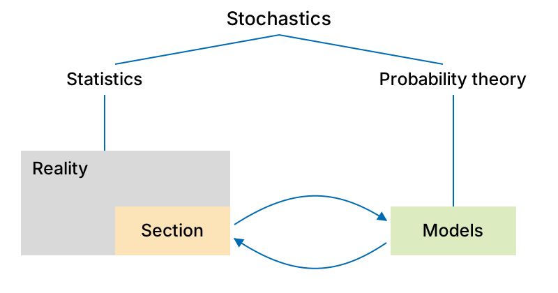
Figure 1:Stochastics as the umbrella term: statistics works on a section of reality, probability theory works on the models.
The two arrows in the middle are what the picture is really saying, and they run in opposite directions. Modelling leads from the section of reality to the models: you observe, collect data and set up a model that fits. Prediction leads from the models back to reality: you calculate within the model and assert something about the world that can be checked. Both directions are needed, and this book walks each of them several times.
As always in computer science, one essential aim is to model a section of reality: to abstract away from that section, to use the model to predict a piece of reality, and to test the model against reality.
We already know logical models of reality: if it rains, the lawn gets wet. If I am hungry and then eat a lot, I am no longer hungry afterwards.
In the notation of propositional logic, the first model is written as an implication. With for “the lawn is wet”, for “it has rained” and for “somebody watered it”, it reads
or, as you would write it in a programming language, (!N) || R || G. The model is useful, but it does not answer the question that actually occupies us when we look at the wet lawn: which of the two was it? Does it rain here often? Has anybody ever watered this lawn at all? Propositional logic can only answer “at least one of the two”.
Statistical models extend this all-or-nothing logic with degrees of plausibility: if the lawn is wet, it is plausible to assume that it rained recently. It is just as plausible that somebody watered the lawn with a garden hose. Which we find more plausible depends on what else we know about reality. If we watch the lawn for longer, we can establish how often each reason leads to a wet lawn, and sharpen our model accordingly.
If we want to calculate with plausibility the way we calculate with Boolean logic, and eventually implement it on a computer, we have to attach numbers to the plausibility values. The real numbers are a suitable abstraction: they are the only Archimedean ordered complete field containing the rationals (and the subalgebra of computable reals inside them has already served us well).
The example shows two things. First, calculating with plausibilities is not as naive as it might first appear; it needs rules. Second, the numbers 20 and 5 are unwieldy because they depend on the observation period: two months of observation would give 40 and 10, though nothing about the matter itself has changed.
We also want plausibility logic to be compatible with classical logic: logically equivalent statements should be equally plausible, and different routes to the plausibility of a statement should arrive at the same result (consistency). To put that into mathematics, let be a finite set of statements whose plausibility we want to assess; an assignment of plausibility is then a map .
Two rules we want in any case. The first is the formula from the example, known as inclusion–exclusion: adding two possibilities counts their overlap twice, so it has to be subtracted once,
The second fixes the problem with the observation period. We normalise so that the plausibility of a statement and that of its negation add up to 1,
since exactly one of the two holds. Every plausibility then lies between 0 and 1, and the absolute length of the observation period drops out: 20 rainy days out of 30 become , whether you count for a month or for a year.
Is that already enough to call these numbers “probability”? Not quite – but almost.
Once these requirements are made precise, one can prove Cox’s theorem: there is a map from the real numbers into the closed interval that takes plausibilities to “probabilities” in such a way that (almost) all the rules of classical probability theory hold. So satisfies the rules
and .
If are finitely many pairwise incompatible (mutually exclusive) statements, then finite additivity holds:
We now approach the modern version of the notion of probability. The sigma-algebra will only be mentioned here; afterwards you may (for the purposes of this course) forget it again.
Digression (optional): the measure problem
For a die or a coin it is reasonably clear how to model the probability, and how to set up a statistical model that we can also implement. In theory, though, the question soon arises of what happens with, say, an experiment repeated infinitely often. That is not a purely theoretical question: we are interested in the asymptotics, that is, in how an experiment behaves, approximately, once it has been repeated often enough.
An infinitely repeated coin toss can be written down as an infinite sequence of 0s and 1s, and on closer inspection that is also a representation of the real numbers in the unit interval – one that can be implemented on a computer insofar as the computer is a Turing machine (in reality the tape is finite, but we can always extend it; or rather, the memory of our computers is bounded, but not by a fixed value).
We would now like to assign a probability to every outcome (every result of the infinitely repeated coin toss) so that , where is the sample space. Moreover, finite additivity should hold for pairwise disjoint subsets :
Another natural requirement is flip invariance: it should make no difference to the probability if I flip exactly the -th coin toss (the -th bit). This is formalised by an operator with
We then expect to hold for every subset .
In 1923 Banach proved, using the axiom of choice, that such a probability can be defined non-constructively – but not uniquely!
If we tighten one of our requirements, from finite additivity to -additivity (say “sigma-additivity” or “countable additivity”), then Vitali had already proved in 1905 that no such map exists at all – so it is impossible to assign probabilities to infinite coin tosses in this way. Why is that, and what does it have to do with -additivity?
Digression (optional): measuring open sets
Here is a very practical definition for any set with a notion of distance (more precisely: a metric space ): a set is called open if around every point there is a distance such that every point with already lies in , that is, . For , finite unions of open intervals are open sets of this kind, which is where the name comes from.
One can now show that the classical - definition of continuity is equivalent to this one: is continuous if the preimages of open sets are open as well.
If we want to define a uniform distribution on the numbers in the interval (as in the infinite coin-toss example), or indeed on all the reals, we already know exactly what we want for intervals: the probability – the measure – of an interval should simply be .
Since every open set in can be written as a countable union of intervals, we know how to assign a measure to the open sets: as the countable sum of the lengths of exactly those intervals. It turns out that a uniform distribution can indeed be defined this way – only that a probability can then no longer be assigned to arbitrary subsets of or . One says that there are non-measurable sets.
From this observation we derive the requirement that our probability be not merely finitely additive but -additive. In the light of Vitali’s theorem we accept that not every subset of is measurable, and content ourselves with singling out a subalgebra of : the measurable sets.
Formalism
So far we have pinned plausibilities to statements: “it rained”, “somebody watered”. Statements are the right object for logic, but they become unwieldy as soon as you want to calculate – even the question of how many different statements there are leads nowhere. The trick of modern probability theory is to replace every statement by the set of situations in which it holds.
To that end we imagine a set of all outcomes under consideration – in the lawn example, say, all the states the world could be in this morning. Every statement about the world splits this set in two: the states in which it is true, and the rest. The statement “the lawn is wet” thus becomes the subset of all world states with a wet lawn, “it rained” becomes and “somebody watered” becomes . Instead of a plausibility for the statement, we are now after a number for the subset.
The gain: the logical connectives become set operations, which we already know our way around.
| Propositional logic | Set logic |
|---|---|
| or , | |
| and , | |
| not , |
The question of how plausible “it rained or somebody watered” is becomes the question of , and “it neither rained nor did anybody water” is , the complement of .
A subset of to which we assign a probability is called an event. It would be convenient to admit every subset of as an event, and for finite that works. In general – this was the lesson of the measure problem – it does not. So we single out a system of “interesting” subsets and require only that it be closed under the operations we have just translated: along with and , the sets , and should lie in , and and in any case. The probability is then a map .
In mathematical language such a system of sets is called a -algebra – the signals that countably infinite unions are allowed too, which we need for passing to the limit. With that we have all the ingredients and can write the definitions down.
Rule of thumb: if it is unclear what the -algebra is supposed to be, it is ; in other words, if it is unclear what a “measurable set” is supposed to be, it simply means “set”.
Compare this with Definition 12.2.5 and Remark 12.2.8 in the German lecture notes “Mathematik für Informatik”, where the special case with finite is assumed.
Rule of thumb: if it is unclear what the -algebras are supposed to be, we picture every map (= function) as measurable. Strictly speaking that is usually false as soon as continuous random variables are involved – and in practice it will not trouble us all the same.
The term random variable is highly misleading: there is neither a variable here nor any randomness. The notion of a measurable map makes sense outside probability theory too, but the notion of a random variable is typically used differently and comes with different syntactic habits. Think of this overloading of the term as an API wrapper that gives us extra syntactic sugar – a map that comes dressed as a random variable can be used like a variable that takes random values. We will lean on this perspective a good deal, and practise it.
We will not go further into measure theory here; defining, say, the general Lebesgue integral takes a certain amount of effort. One thing, though, is worth recording because of the applications in computer science, and in machine learning in particular: whereas the Riemann integral approximates with the areas of rectangles, the Lebesgue integral approximates the function itself by step functions.
This lets a great many statements be proved by proving them for step functions (the construction of the Lebesgue integral among them). It also yields far-reaching universality statements whenever a model of computation can approximate step functions to arbitrary accuracy – which is how the universality of neural networks can be seen; the course Introduction to Deep Learning works this out (universal approximation).
Finally, it should be said that there is a legitimate objection to this formalism: a computer can only implement constructive mathematics, and neither the law of the excluded middle nor the axiom of choice is implementable. In that logic, though (the constructivist, so-called intuitionistic one), every subset of a metric space may be called measurable, precisely because the non-measurable subsets cannot be constructed. That makes some things easier, but a great many things impossible. So we content ourselves with knowing how to read texts that use the usual formalism, and with having a good excuse at hand for not engaging with it any further.
So you can now pick up a probability textbook, find a theorem saying “let X be a set with a -algebra ...” and, for the time being, read past the -algebra part, since in practice you will not run into non-measurable sets (those that are not in the system of sets called a -algebra). In other words: as a first approximation, imagine that “measurable” is no restriction at all. What we should take away from this chapter at the very least is the notion of a random variable, the rules of calculation for probability measures , and the important example of the uniform distribution.
If you would like to approach stochastics through interactive playthings as the course goes on, Random Services is just the thing for you. If you prefer things elegant and visual, Seeing Theory will accompany you through the stochastics part of the course.