Programming with stochastics: simulating random experiments - Data Science Lecture Notes from Konrad Völkel

Let us look briefly at how to simulate samples from random experiments in Python.

Python constructs used: Modules/import, Functions/def, Length/len, Sets/set, Generator expression, Range, Assertion/assert, Counting/Counter

Implementing a probability measure¶

from fractions import Fraction

def P(A, Omega):
    """The probability of the event A,
       given equally likely outcomes from a sample space Ω."""
    return Fraction(len(A & Omega), len(Omega))

Now we use it to program a throw of a die:

Omega = {1, 2, 3, 4, 5, 6}
even = set((x*2 for x in range(1,4)))
print("Even numbers of pips:",even)

print("Probability of an even number of pips:", P(even, Omega))

Even numbers of pips: {2, 4, 6}
Probability of an even number of pips: 1/2

That gives us the probability measure. To draw a sample, though, we still need to get the “randomness” from somewhere.

Importing randomness¶

Python’s random module is an interface to pseudo-random numbers. The function random.random is a Mersenne Twister implemented directly in C. If you need “real” random numbers, for cryptography say, there is the secrets module. The seed of the Mersenne Twister can be set, and should be, so that random simulations are reproducible.

from random import random as r
help(r)
print("1", r())
print("2", r())

import random
random.seed(1)
very_random = r()
print("3", very_random)
assert very_random == 0.13436424411240122
print("4", r())
random.seed(1)
print("5", r())

Help on built-in function random:

random() method of random.Random instance
    random() -> x in the interval [0, 1).

1 0.4874556251922124
2 0.14064250428300507
3 0.13436424411240122
4 0.8474337369372327
5 0.13436424411240122

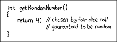
Randall Munroe, xkcd 221 “Random Number” (CC BY-NC 2.5)

From a (pseudo-)random number between 0 and 1 (note: possibly 0, but never 1) we can generate random throws of a die:

from math import floor
def transform_unit_to_dice(x):
    return floor(1 + 6*x)

assert list(range(1,7)) == [transform_unit_to_dice((x-1)/6)
                            for x in range(1,7)]

N = 100
throws = [transform_unit_to_dice(r()) for n in range(N)]
print(throws)

[6, 5, 2, 3, 3, 4, 5, 1, 1, 6, 3, 5, 1, 3, 5, 2, 6, 6, 1, 1, 4, 6, 3, 2, 3, 1, 2, 3, 3, 2, 2, 2, 3, 2, 1, 6, 4, 4, 2, 6, 6, 1, 2, 5, 5, 6, 3, 5, 5, 2, 4, 6, 6, 4, 4, 1, 2, 5, 3, 2, 4, 5, 5, 3, 3, 4, 5, 4, 3, 3, 1, 1, 5, 6, 4, 3, 2, 4, 6, 5, 4, 6, 2, 4, 6, 4, 3, 2, 4, 6, 1, 5, 5, 6, 5, 5, 4, 4, 3, 1]

Let us count how often each number of pips came up. The relative frequency is the count divided by $N$ :

from collections import Counter

frequencies = Counter(throws)
for pips in range(1, 7):
    print(pips, "came up", frequencies[pips], "times, relative frequency", frequencies[pips] / N)

1 came up 13 times, relative frequency 0.13
2 came up 16 times, relative frequency 0.16
3 came up 18 times, relative frequency 0.18
4 came up 18 times, relative frequency 0.18
5 came up 18 times, relative frequency 0.18
6 came up 17 times, relative frequency 0.17

To spare you programming such transformations over and over, there are also random.randint(1,6), random.choice(range(1,7)) and random.randrange(1,7). Here randint is shorthand for the corresponding randrange, and choice is somewhat more general.

But let us put on record what we have done: starting from a uniformly distributed “random variable” $X=$ random.random with values in $[0,1)$ , we constructed and implemented a map $t =$ transform_unit_to_dice with values in $\Omega := \{1,2,3,4,5,6\}$ , and $t(X)$ is uniformly distributed. The mathematical map $t \colon [0,1) \to \Omega$ is a random variable, and we treat the composition $t \circ X$ as the random variable that models the die.

Now you might object that random.random() takes no parameter at all, so it is not a mathematical map from a domain into the set $[0,1)$ . In fact we have to imagine it as a map $X \colon \Omega' \to [0,1)$ , with some probability measure or other defined on $\Omega'$ in such a way that $X$ induces the uniform distribution on $[0,1)$ . The set $\Omega'$ plays no concrete role for us – it is where “the randomness comes from”, and the notation random.random() already tells us that we are not plugging in any particular element of $\Omega'$ , but drawing one pseudo-randomly and plugging that into $X$ .

Larger samples¶

The function random.sample(population, k) draws a sample of size $k$ from a population (an urn) without replacement, so the elements drawn are pairwise distinct. For $k=1$ this amounts to a uniform distribution on the population. The function random.choices(population, weights=None, *, cum_weights=None, k=1) draws from the population $k$ times with replacement (and lets you assign weights instead of assembling a suitable population).

Looking ahead¶

The relative frequencies we counted in this notebook for the numbers of pips $1,\dots,6$ are estimates of the die’s probabilities $p(1),\dots,p(6)$ . In the next chapter we will call the function $p$ the probability mass function (pmf) of the random variable ‘number of pips’, and make the throw of a die our first statistical model.