The Gaussian normal distribution and the central limit theorem

Approximating the binomial distribution¶

Consider a sequence of Bernoulli distributed random variables $X_i$ with the same parameter $p$ , and let $S_n := \sum_{i=1}^n X_i$ be the sum of the first $n$ of them. From the chapter The most important discrete distributions we know that $S_n \sim \operatorname{Bin}(n,p)$ : the sum is binomially distributed. As a reminder, this means the pmf of $S_n$ is $p(k) = \binom{n}{k}p^k(1-p)^{n-k}$ .

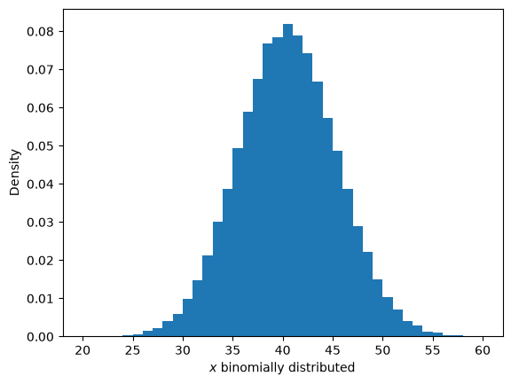
For the concrete values $n=100,\ p=0.4$ , a histogram of 100000 samples looks something like this:

import numpy as np
from scipy.stats import binom, norm
from matplotlib import pyplot as plt
np.random.seed(123123)
binom_samples = binom.rvs(n=100,
                          p=0.4,
                          size=100000)
plt.hist(binom_samples, bins=40, density=True)
plt.xlabel("$x$ binomially distributed")
plt.ylabel("Density")
plt.show()

Since large samples always produce this shape, whatever $p$ may be (try it out!), you might suspect that the distribution can be approximated by a function that is easier to compute than the binomial coefficients $\binom{n}{k} = \frac{n!}{k!(n-k)!}$ .

Aside: there is in fact Stirling’s formula for approximating the factorial,

n! \approx \sqrt{2\pi n} {\left(\frac{n}{e}\right)}^n

(1)

which for binomial coefficients gives us directly: $\binom{n}{k} \approx \frac{\sqrt{n}}{\sqrt{2\pi}\sqrt{k}\sqrt{n-k} } \frac{n^n}{k^k {\left(n-k\right)}^{(n-k)} }$

With this, an approximation can be proved (though it is not entirely easy):

P(S_n = k) = \binom{n}{k}p^k(1-p)^{n-k} \sim \frac{1}{\sqrt{np(1-p)}} \frac{1}{\sqrt{2\pi}} e^{-\frac{x^2}{2}} \quad \text{ for } n \to \infty

(2)

where on the right-hand side the sequence $x=x_n$ with $x_n = x_n(k) = \frac{k-np}{\sqrt{np(1-p)}}$ has to be substituted for $x$ . The symbol $\sim$ means asymptotically equal: the quotient converges to 1.

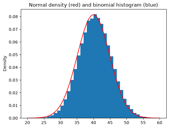
The approximation is useful because we can now tabulate the function $e^{-\frac{x^2}{2}}$ and read off concrete values for any given $n,p$ – considerably more efficient than computing binomial coefficients. The whole observation is known as the theorem of de Moivre–Laplace, and for now it serves as our motivation for examining the function $e^{-\frac{x^2}{2}}$ more closely.

An integral¶

To turn the function $e^{-\frac{x^2}{2}}$ into a probability density, its integral has to come out as 1. Since it will be very useful later, we compute a slightly more general integral right away:

Proof

The square root on the right-hand side suggests squaring both sides of the equation. We then keep rewriting the left-hand side until we can switch an integral over $\mathbb{R}^2$ to polar coordinates and, after a substitution, find antiderivatives easily:

\begin{aligned} & {\left( \int_{-\infty}^\infty e^{-\frac{x^2}{2v}} dx \right)}^2 \\ =& {\left( \int_{-\infty}^\infty e^{-\frac{x^2}{2v}} dx \right)}{\left( \int_{-\infty}^\infty e^{-\frac{y^2}{2v}} dy \right)} \\ =& \int_{-\infty}^\infty e^{-\frac{x^2}{2v}} {\left( \int_{-\infty}^\infty e^{-\frac{y^2}{2v}} dy \right)} dx \\ =& \int_{-\infty}^\infty {\left( \int_{-\infty}^\infty e^{-\frac{x^2}{2v}} e^{-\frac{y^2}{2v}} dy \right)} dx \\ =& \int_{-\infty}^\infty {\left( \int_{-\infty}^\infty e^{-\frac{x^2+y^2}{2v}} dy \right)} dx \\ =& \int_{\mathbb{R}^2} e^{-\frac{x^2+y^2}{2v}} d(x,y) \\ =& \int_{0}^\infty \int_{0}^{2\pi} r e^{-\frac{r^2}{2v}} d\phi dr \\ =& \int_{0}^\infty r e^{-\frac{r^2}{2v}} \int_{0}^{2\pi} d\phi dr \\ =& \int_{0}^\infty r e^{-\frac{r^2}{2v}} [\phi]_0^{2\pi} dr \\ =& \int_{0}^\infty r e^{-\frac{r^2}{2v}} 2\pi dr \\ =& 2\pi \int_{0}^\infty e^{-\frac{r^2}{2v}} r dr \\ =& 2\pi \int_{0}^{-\infty} e^u (-v)du \\ =& 2\pi v \int_{-\infty}^{0} e^u du \\ =& 2\pi v [e^u]_{-\infty}^{0} \\ =& 2\pi v. \end{aligned}

(4)

Since integrals turn up rather often in statistics, it is worth working through this calculation and seeing exactly what happens at each step, and why.

The one-dimensional normal distribution¶

x = np.linspace(20,60,100)
plt.hist(binom_samples, bins=40, density=True)
plt.plot(x, norm(loc=40, scale=np.sqrt(24)).pdf(x), color="red")   # expected value n p = 40, variance n p (1-p) = 24
plt.ylabel('Density')
plt.title('Normal density (red) and binomial histogram (blue)')
plt.show()

Proof

We substitute the density for $X$ into the formula for $\mathbb{E}(X)$ and transform the integral over $x$ into an integral over $x + \mu$ :

\begin{aligned} \mathbb{E}(X) &= \int_{-\infty}^{\infty} x\phi(x) dx \\ &= \int_{-\infty}^{\infty} x \frac{1}{\sigma\sqrt{2\pi}} e^{-\frac{(x-\mu)^2}{2\sigma^2}} dx \\ &= \frac{1}{\sigma\sqrt{2\pi}} \int_{-\infty}^{\infty} x e^{-\frac{(x-\mu)^2}{2\sigma^2}} dx \\ &= \frac{1}{\sigma\sqrt{2\pi}} \int_{-\infty}^{\infty} (x+\mu) e^{-\frac{x^2}{2\sigma^2}} dx \\ &= \frac{1}{\sigma\sqrt{2\pi}} \left( \left( \int_{-\infty}^{\infty} x e^{-\frac{x^2}{2\sigma^2}} dx \right) + \mu \left( \int_{-\infty}^{\infty} e^{-\frac{x^2}{2\sigma^2}} dx \right) \right) \\ &= \frac{1}{\sigma\sqrt{2\pi}} \left( \left( \int_{-\infty}^{\infty} x e^{-\frac{x^2}{2\sigma^2}} dx \right) + \mu \sigma\sqrt{2\pi} \right) \\ &= \mu + \frac{1}{\sigma\sqrt{2\pi}} \left( \int_{-\infty}^{\infty} x e^{-\frac{x^2}{2\sigma^2}} dx \right) = \mu.\\ \end{aligned}

(6)

The expression after the $\mu +$ is simply 0, because the function is point-symmetric about 0 (the factor $x$ is obviously odd, and the other factor depends only on $|x|$ ).

The variance is handled in exactly the same way, by simplifying this expression:

\begin{aligned} \mathbb{V}(X) &= \int_{-\infty}^{\infty} x^2\phi(x) dx - {\left( \mathbb{E}(X) \right)}^2 \\ &= \int_{-\infty}^{\infty} x^2\frac{1}{\sigma\sqrt{2\pi}} e^{-\frac{(x-\mu)^2}{2\sigma^2}} dx - \mu^2. \end{aligned}

(7)

After the same substitution $x \to x + \mu$ and expanding $(x+\mu)^2$ , what is left is $\frac{1}{\sigma\sqrt{2\pi}} \int x^2 e^{-x^2/2\sigma^2}\,dx$ (the mixed term is again odd, and the $\mu^2$ term cancels), and integration by parts with $u = x$ , $v' = x e^{-x^2/2\sigma^2}$ yields $\sigma^2$ for it; we leave the details to you.

Standardisation is a special case of a more general statement that you will need all the time:

Proof

Idea: Expected value and variance follow from the rules of calculation in the chapter Expected value and variance. That the shape is preserved can be read off the density: if a random variable $X$ has density $p_X$ , then $Y = aX+b$ has density

p_Y(y) = \dfrac{1}{|a|}\, p_X\!\left( \dfrac{y-b}{a} \right)

(9)

(the transformation formula: the factor $\frac{1}{|a|}$ makes sure the integral comes out as 1 again). Substituting the normal density, the exponent becomes $-\frac{((y-b)/a - \mu)^2}{2\sigma^2} = -\frac{(y - (a\mu+b))^2}{2a^2\sigma^2}$ and the prefactor $\frac{1}{|a|\sigma\sqrt{2\pi}}$ – exactly the density of $\mathcal{N}(a\mu+b, a^2\sigma^2)$ .

Two special cases are worth remembering. With $a = \frac1\sigma$ and $b = -\frac\mu\sigma$ we get the standardisation from above. And conversely: if $Z \sim \mathcal{N}(0,1)$ , then $\sigma Z + \mu \sim \mathcal{N}(\mu,\sigma^2)$ – so every normal distribution arises from the standard normal distribution by stretching and shifting. That is exactly how they are generated on a computer, too: mu + sigma * rng.standard_normal(n) needs only one random number generator for all normal distributions. The chapter The multivariate normal distribution takes this as its starting point: there the same construction is carried out with a matrix instead of a number.

We also use the fact that the sum of independent random variables with densities $f,g$ again has a density, namely the convolution $f \ast g$ . Rather than introduce and prove that rigorously, we merely record the result for normal distributions, which can be checked using the convolution.

Even to state this theorem precisely, we need a notion of entropy for continuous distributions. Rather than set that up now, we return to it later, when we also discuss relative entropy, its continuous version and likelihood.

Expected value and variance follow from the rules of calculation in the chapter Expected value and variance; the remarkable part is that the shape is preserved too – the sum is not just some distribution with these moments but a bell curve again. That is far from obvious: the sum of two uniformly distributed variables is triangularly distributed, not uniformly distributed. The normal distribution is said to be stable under convolution. The chapter on the multivariate normal distribution shows the generalisation: there the same holds for dependent $X, Y$ too, as soon as they are jointly normally distributed, with an extra covariance term in the variance.

What matters, though, is the theorem’s take-home message: if nothing is known about a continuous distribution on the real numbers beyond its expected value and variance, the corresponding normal distribution is the most sensible assumption. In this sense the normal distribution is a good continuous substitute for the discrete uniform distribution, but now on all of $\mathbb{R}$ (the normal distribution has support $\mathbb{R}$ ).

The restriction to support $\mathbb{R}$ is no formality here; it is the actual modelling assumption. If the support is known more precisely, a different distribution has maximal entropy – and is hence the most sensible assumption:

Support	what else is known	distribution with maximal entropy
$\{1,\dots,n\}$	nothing	discrete uniform distribution, $p(k) = \frac1n$
$[a,b]$	nothing	continuous uniform distribution, $f(x) = \frac{1}{b-a}$
$[0,\infty)$	expected value $\mu$	exponential distribution, $f(x) = \lambda e^{-\lambda x}$ with $\lambda = \frac1\mu$
$\mathbb{R}$	expected value and variance	normal distribution
$[a,b]$	expected value and variance	truncated normal distribution (`scipy.stats.truncnorm`)

The profiles of the three continuous distributions are in the chapter The most important continuous distributions, that of the discrete uniform distribution in the chapter The most important discrete distributions. The truncated normal distribution is exactly what it sounds like: a normal distribution whose density is set to 0 outside $[a,b]$ and renormalised inside. You need it when a quantity is bounded by its very nature – proportions between 0 and 1, readings at the display limit of an instrument – and a normal model would otherwise put probability mass where no values can occur at all.

The pattern behind this is always the same: maximal entropy means “assume as little extra as possible”. What you know goes in as a constraint; everything else you leave to chance.

The central limit theorem¶

The letter $Z$ is a reminder that $Z_N$ is the sum $S_N = \sum_{i=1}^N X_i$ we looked at above for Bernoulli variables, normalised to expected value 0 and variance 1.

Convergence in distribution means that the cumulative distribution function of $Z_N$ converges to that of a standard normal distribution.

There are also weaker versions of this theorem that allow certain dependencies among the $X_i$ .

Two concrete examples: the error in position fixing with GNSS systems such as GPS is normally distributed (even though the atmospheric disturbances that make the value less accurate are not). In the industrial manufacture of components, likewise, sources of error throughout the production process add up to a normal distribution in the end – one whose variance has to be kept small enough for the component to do its job. A Lego brick, for instance, must not deviate too much from an identically built Lego brick, or the structure will not hold together properly afterwards.

Remark

The standard error. The application that matters most to us: the mean $\overline{X}_N$ of a sample of size $N$ is itself a (scaled) sum, and hence approximately normally distributed for large $N$ , with expected value $\mu$ and standard deviation $\sigma/\sqrt{N}$ . This standard deviation of the sample mean is called the standard error. Since a normally distributed quantity deviates from its expected value by less than 1.96 standard deviations with probability $95\,\%$ , the true expected value lies in the interval $\overline{X}_N \pm 1.96\,\sigma/\sqrt{N}$ for about $95\,\%$ of all samples. That is sharper than Chebyshev’s inequality from the chapter Expected value and variance, which guarantees only $75\,\%$ for two standard errors, and it is the recipe by which the chapter Statistical tests reasons from the sample to the population. Titanic example: of 314 women, $74.2\,\%$ survived; the standard error of this proportion is $\sqrt{0.742 \cdot 0.258 / 314} \approx 0.025$ , so the interval is about $74 \pm 5$ percentage points.

Aside: the speed of the convergence can be estimated too, which tells us how good the approximation by a normal distribution is:

Theorem (Berry–Esseen)

There exists a constant $C$ with $0.41 \le C \le 0.48$ and the following property:

If $X_i$ is a sequence of iid random variables with expected value 0 and variance $\sigma^2$ whose third absolute moments $\mathbb{E}|X_i|^3 = \rho < \infty$ also exist, and if we write $F_N$ for the cumulative distribution function of $Z_N = \frac{1}{\sigma\sqrt{N}} \sum_{i=1}^N X_i$ and $\Phi$ for that of the standard normal distribution $\mathcal{N}(0,1)$ , then for all $N$ :

\sup_{x \in \mathbb{R}} \left| F_N(x) - \Phi(x) \right| \ \leq\ \dfrac{C\rho}{\sigma^3 \sqrt{N}}.

(11)

The exact value of $C$ is not known; the bounds given are the current state of research. So for concretely known $\sigma,\rho$ we can always find an $N$ that makes the left-hand side as small as we like. In other words: for any desired accuracy, we can compute how many of the iid random variables have to be added up (and scaled) for $Z_N$ to be approximated by a standard normal distribution.

Naturally, if the expected value is not 0, a variant follows as a corollary (as with the central limit theorem), with convergence to $\mathcal{N}(\mu,1)$ – and with a different rescaling, to $\mathcal{N}(\mu,\sigma^2)$ as well. In practice it looks more like this: every unknown error term is modelled by a normal distribution whose expected value and variance are estimated empirically.

A practical example: The “ $N \ge 30$ ” myth¶

Many textbooks, statistics courses and analysis protocols offer a rule of thumb: from $N = 30$ on you may work with a normal distribution. The rule is so widespread that it is rarely questioned – and in that form it is wrong. And Berry–Esseen tells us why.

The bound above reads $\frac{C\rho}{\sigma^3\sqrt{N}}$ . In it, $N$ appears only under a square root; the decisive quantity is the factor $\rho/\sigma^3$ , the third absolute moment relative to the cube of the standard deviation – a measure of how skewed the individual random variable is. For a symmetric distribution this factor is small; for a skewed one it can be arbitrarily large, and then $N = 30$ is simply not enough.

The most important case in practice is a binary feature: “side effect occurred yes/no”, “click yes/no”, “survived yes/no”. Such a feature is Bernoulli distributed with parameter $p$ , and for it we can compute the factor. For $X \sim \operatorname{Bernoulli}(p)$ , centred to have expected value 0,

\sigma^2 = p(1-p), \qquad \rho = \mathbb{E}\left|X - p\right|^3 = p(1-p)\left[(1-p)^2 + p^2\right],

(12)

hence

\dfrac{\rho}{\sigma^3} = \dfrac{(1-p)^2 + p^2}{\sqrt{p(1-p)}}.

(13)

For a balanced feature, $p = 0.5$ , this is exactly 1, and the Berry–Esseen bound at $N = 30$ comes out (with $C \approx 0.44$ ) at $0.44/\sqrt{30} \approx 0.08$ : the cumulative distribution functions differ by at most eight percentage points – usable. For a rare event, $p = 0.01$ , by contrast, the same factor is $\approx 9.85$ and the bound at $N = 30$ becomes

\dfrac{0.44 \cdot 9.85}{\sqrt{30}} \approx 0.79.

(14)

A bound of 0.79 on the deviation between two cumulative distribution functions that both lie between 0 and 1 says nothing at all – it is useless. Only at $N = 1000$ does it drop to $\approx 0.14$ . (The Berry–Esseen bound is an upper bound; the actual error may be smaller. But a rule of thumb that cannot even be justified from above is not one you should use.)

So the difference from the $N \ge 30$ rule is not academic: for an event that hits one case in a hundred, the correct threshold is 33 times higher. That is exactly the situation with rare side effects in medical studies.

fig, (ax1, ax2) = plt.subplots(1, 2, figsize=(12, 4))

for ax, n in ((ax1, 30), (ax2, 1000)):
    p = 0.01
    k = np.arange(0, int(n * p + 4 * np.sqrt(n * p * (1 - p))) + 2)
    ax.bar(k, binom(n, p).pmf(k), label="Binomial distribution", alpha=0.7)
    xs = np.linspace(k.min() - 1, k.max(), 200)
    ax.plot(xs, norm(loc=n * p, scale=np.sqrt(n * p * (1 - p))).pdf(xs),
            color="black", label="Normal approximation")
    np_text = f"{n * p:g}"
    ax.set_title(f"$N = {n}$, $p = 0.01$   ($Np = {np_text}$)")
    ax.set_xlabel("Number of successes")
    ax.legend()

plt.show()

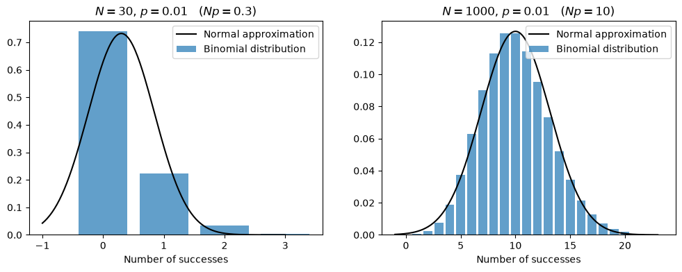
On the left, at $N = 30$ , almost all the probability mass sits on the values 0 and 1 – the distribution is cut off at zero and heavily skewed to the right, while the normal approximation runs placidly off into negative territory and spreads probability where there are no outcomes at all. On the right, at $N = 1000$ , the Laplace condition is just satisfied, with $Np = 10$ , and the bell shape is recognisable.

The moral is more general than the example: a rule of thumb that names only the sample size and says nothing about the distribution cannot work. What counts is the ratio of skewness to sample size.

Approximating the binomial distribution¶

An integral¶

The one-dimensional normal distribution¶

The central limit theorem¶

A practical example: The “N≥30N \ge 30N≥30” myth¶

A practical example: The “ $N \ge 30$ ” myth¶