Exploratory data analysis leaves us with hypotheses about which relationships are hidden in the data. When we build systems with machine learning we have a great many decisions to make: whether we may treat a variable as normally distributed, say, or whether two groups or clusters have roughly the same distribution or very different ones.
Tests appear here in two quite different roles, and it helps to keep them apart. In exploratory analysis they are one tool among many and answer questions such as “Is this attribute normally distributed?”, “Do samples A and B have the same distribution for this attribute? The same mean?” – the answer then decides the next step of the analysis, for instance whether a method that presupposes normality may be used at all. In communicating results, by contrast, they are the argument itself: “The test shows that the groups have different distributions, so we use a mixture model” (see Expectation Maximization). In the first role you may test generously, in the second you may not; the section Significance at the end of this chapter explains why.
Strictly speaking, statistical tests are not part of “machine learning”, but in the running order of the lecture course this is where they fit naturally.
A test can be read as an estimator that estimates not a single value but a whole range of possible values, followed by a decision rule that interprets the estimate in the light of a hypothesis. We will treat the subject only superficially – just far enough to judge what a test can achieve and where the limits of statistical tests lie – but before that we look at what the difference between single values and ranges of values means for communicating scientific results, data science results included.
Prediction intervals
By way of motivation we look at the figure Figure 1 and then set it against Figure 2.
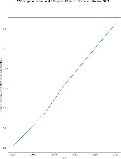
Figure 1:Global warming, projection (A2r scenario at 970 ppmv, IIASA 2009)
The figure shows the projection of a statistical model for global warming – given here as the temperature change relative to the pre-industrial level, defined as the mean temperature of the years 1850 to 1900 – on the assumption that the CO2 content of the atmosphere rises to 970 ppmv (parts per million by volume; for comparison, 30 May 2022: 421 ppmv, and 1900: 296 ppmv). For context: the Paris climate agreement sets a limit of 1.5°C or 2°C – not by 2040, but by 2100.
Let us look at this figure with a data scientist’s eyes: what is there to criticise?
A common objection to models and figures of this kind is that things could turn out this way, but just as easily quite differently – these are only theoretical models, after all. The figure expresses a certainty about the course of the curve that cannot possibly exist, which makes the claim “this is how it will be” implausible from the outset. Granted, what it means to say is “this is how it could be”, but on its own that is about as useful as “it might rain or it might stay dry”.
To make decisions on the basis of a statistical prediction we also need to know how plausible it is. For comparison, look at Figure 2, a figure from the IPCC report SR15, Summary for Policymakers, Figure 1 a) Allen et al. (2018):
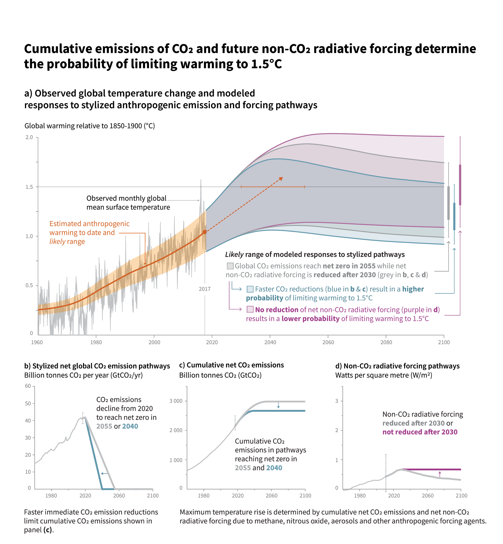
Figure 2:Global warming, projection (IPCC SR15, Fig. 1)
To read this figure properly we also need to know the IPCC Calibrated Language, or more precisely the Likelihood scale (AR4 and AR5 here refer to the ‘assessment reports’ that appeared before the special report on 1.5°C):
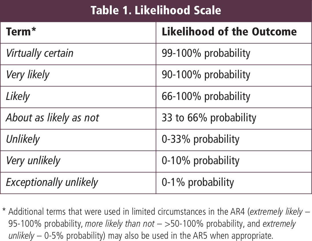
Figure 3:The Likelihood scale of the IPCC Calibrated Language Allen et al. (2018).
Now we can see that the grey shaded area is where the actual measurements will lie with probability at least (according to the model). With that information we can judge far better what warming to expect even if we ‘get lucky’, and how bad it could get if we ‘are unlucky’. Strictly speaking, the grey shaded area is a prediction interval: the range in which the actual future value is presumed to lie with high probability. Closely related is the confidence interval for a parameter: an interval computed from the sample and constructed so that in (say) 95% of all samples it covers the true parameter.
For the mathematical theory of set estimators and confidence intervals we refer you to the statistics lectures. In what follows our main aim is to understand the notion of a test well enough to judge whether a claimed interpretation of a statistical test is serious. Once we can do that, we also want to recognise the situations in which a hypothesis test can deliver useful insight. Above all, that means getting clear about the notion of significance.
From the sample to the population
Before we define tests, let us be clear about what we actually want. Every summary measure from the exploratory analysis – mean, proportion, median, correlation coefficient – is computed on a sample. What we are interested in is the population the sample came from: all passengers, all customers, all the measurements that could have been made. A different sample would have yielded a different number. Inferring from the sample to the population therefore always takes three steps:
Estimate: compute the summary measure from the sample (the proportion, the mean, the difference of two means).
State the uncertainty: an interval in which the population’s summary measure plausibly lies. A number without an interval is not an inference about the population but a description of the sample.
Decide: hold the question you had up against the interval. “Is the coin fair?” means: does lie in the interval? “Do women survive more often?” means: does 0 lie in the interval for the difference?
There are two routes to step 2.
The standard error. By the central limit theorem the mean of a sample of size is approximately normally distributed with standard deviation , the standard error. In of samples the population mean then lies in the interval
where is replaced by the sample standard deviation. For a proportion we have . Coin-toss example: with 45 successes in 100 tosses, and the standard error is , so the interval is roughly . The lies inside it, so the coin could be fair. To reject that, the interval would have to be narrower, and it shrinks only with : halving the width takes four times the sample. (With the cruder Chebyshev inequality in place of the normal approximation one gets an interval of and a required sample of over 2000 tosses; that calculation is in the section Looking ahead: confidence intervals below.)
The bootstrap. For summary measures that have no formula, or whose formula you do not know, you pretend that the sample is the population: draw from it, with replacement, a new sample of the same size, compute the measure, and repeat many thousands of times. The spread of these bootstrap measures estimates the spread of the measure across real samples, and the 2.5 and 97.5 percentiles give a 95% interval. With the arrays survived and sex from the chapter Titanic EDA:
rng = np.random.default_rng(0)
f = survived[sex == 'female']
m = survived[sex == 'male']
difference = f.mean() - m.mean()
bootstrap = np.array([rng.choice(f, len(f)).mean() - rng.choice(m, len(m)).mean()
                      for _ in range(10000)])
print(difference, np.percentile(bootstrap, [2.5, 97.5]))
0.553 [0.495 0.609]The women’s survival rate is 55 percentage points above the men’s, and even at the unfavourable end of the interval still 50. The 0 lies far outside: the difference is no accident of the sample. scipy.stats.bootstrap does the same thing in one line, with better-corrected percentiles.
What the recipe assumes. Both routes assume that the sample is a random sample from the population, that is, that every row of the population had the same chance of ending up in the sample. The Titanic list is a random sample of exactly one population: the passengers of that ship (and even then only the Kaggle extract). About other shipping disasters the interval says nothing, however narrow it is. Anyone who runs a survey on campus and wants to draw conclusions about all students has the same problem, and no sample size in the world cures it.
A statistical test, the subject of this chapter, is step 3 made formal: a rule, fixed in advance, that decides from the sample whether a hypothetical value is still plausible. The z-test and the t-test below are exactly the standard-error calculation above, read the other way round: instead of asking whether lies in the interval around , they ask how many standard errors is away from .
Looking ahead: confidence intervals
But what is our confidence – our trust – in this? Do we still regard values far from as halfway plausible, or can we pin down a very narrow range around that we hold to be plausible? In the concrete example with the estimate , would still be halfway plausible?
We now want to construct intervals with as small as possible, such that the condition on a confidence region from the definition is satisfied:
In words: we are to determine (as a function of , and as small as possible) so that holds for fewer than a proportion of the possible samples . With , say (a common choice), that means our estimation error exceeds in only 5% of samples.
The shape of this inequality may remind you of Chebyshev’s inequality, which we met right after introducing the variance. For the estimator it says
Naturally we would like to take and choose as a function of so that nothing but is left on the right-hand side. We have , which annoyingly still depends on – exactly the thing we do not know!
So we bound (easy to check: equality at , strict inequality everywhere else).
Putting it all together, is well chosen if
In our concrete example, with and , does what we want. For us that means: for the concrete observation , not only the point estimate is plausible; we also regard roughly and as plausible. So the coin could well be fair, and we have merely caught an unlucky observation.
So confidence intervals obtained from Chebyshev’s inequality are very wide. There are several better (and considerably more complicated!) methods for obtaining narrower ones.
But we also see a simple relationship between and : making smaller (that is, demanding more certainty) makes bigger; making bigger (taking larger samples) makes smaller.
With that we can compute, for instance, how large the sample has to be before we can say with certainty at least that our coin is not fair. Again, concretely, suppose one sample has given us the estimate .
and putting in , the sample has to be larger than 2000 before we can reject the claim that the coin is fair. With a cleverer procedure for determining narrower confidence intervals, a smaller sample would do.
We now want to know how well estimates – how far does our confidence, our trust, reach?
The random variable is normally distributed, with mean and standard deviation . The estimation error, measured with the standard deviation of as the ‘unit’, is
and is therefore standard normally distributed. The trouble with this quantity is that we do not actually know , and yet we would like to look at the error of our estimate of . So we have to replace by its estimate .
The random variable ‘sample variance’ is distributed so that follows a distribution with degrees of freedom (a special case of the gamma distribution).
The probability density function of the distribution need not concern us at the moment (and in particular is not part of the course proper); for completeness, here it is:
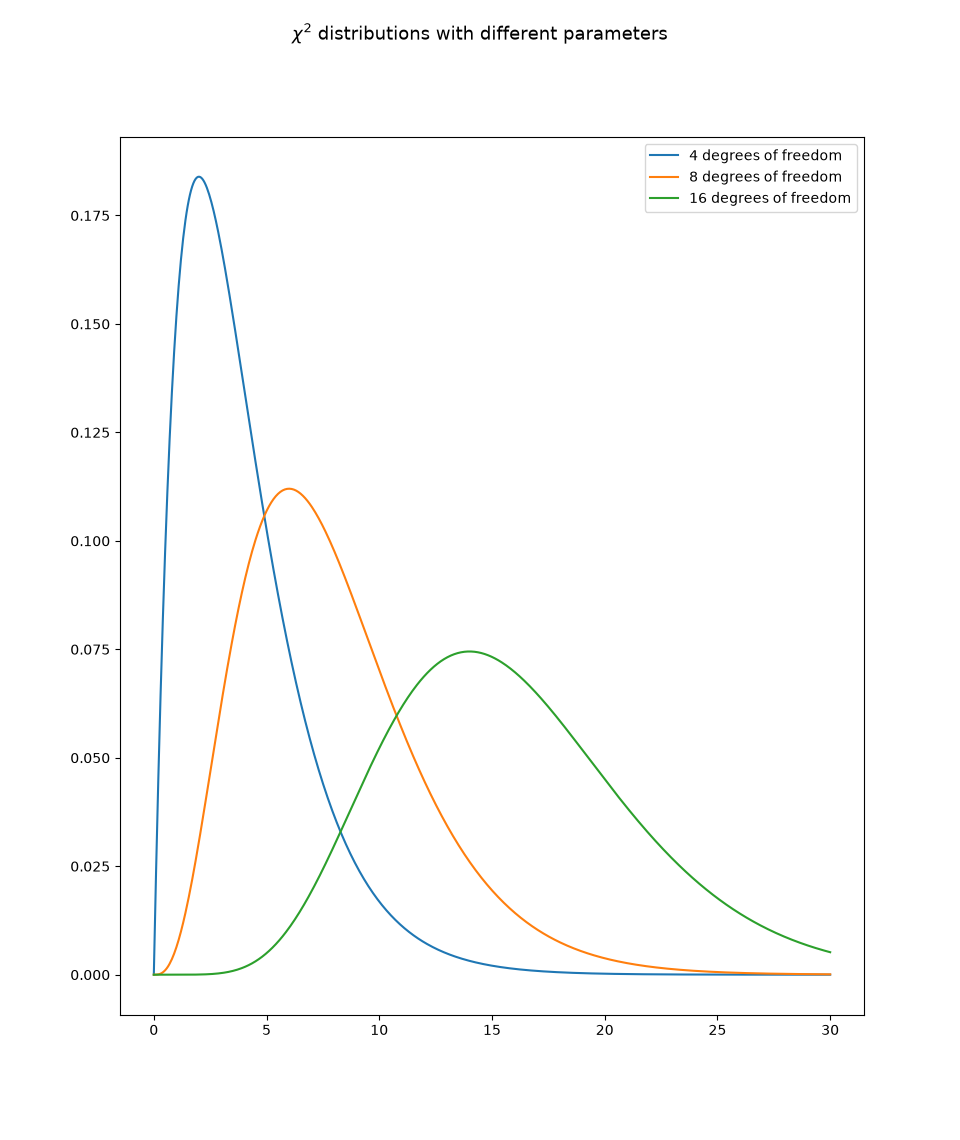
Figure 4:Chi-squared distributions with various parameters (degrees of freedom)
The difference between the estimated mean and the actual expected value, measured with the sample standard deviation as the ‘unit’, is the estimated estimation error , the statistic we look at next:
The random variable follows a Student t distribution, which at first glance looks like a normal distribution but has heavier tails: it takes values far from the expected value with higher probability. Its only parameter is the number of degrees of freedom , here . For of at least 3 the expected value is 0 and the variance is .
The probability density function of the Student t distribution matters little to us for now; for completeness, this is what it looks like:
where is the beta function and the gamma function , defined on all of , interpolates so that always holds (all of which we may promptly forget again).
As the Student t distribution converges to the standard normal distribution. So the gap between the t distribution and the normal distribution encodes exactly the uncertainty that a small sample brings with it.
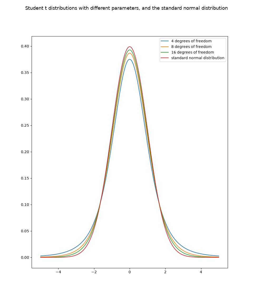
Figure 5:Student t distributions with various parameters (degrees of freedom)
We are now interested in where the probability of a large estimation error is small. Now this estimation error does not depend on – more precisely, is independent of . That may seem counter-intuitive, since appears in the formula, but it is true all the same. The statistic is said to be distribution-free.
For a given we now choose as the -quantile of the distribution with degrees of freedom, that is, the number with ; by the symmetry of the distribution we then have . This used to be looked up in a table; today we ask the computer (scipy.stats.t.ppf(1 - alpha/2, n - 1)).
Then, with , a confidence interval for is given by
So we see that constructing a confidence region can get complicated quickly. On the other hand, the procedure described here (standardise, then apply the quantile transformation) carries over to other situations as well – which we would rather leave to the statisticians.
By approximating the binomial distribution with a normal distribution and then applying the method just discussed for confidence intervals of a normal distribution, one also gets better confidence intervals for a binomial distribution – though here again more complicated procedures yield considerably better ones.
It is enough for us to know where the distribution and the Student t distribution come from; the concrete probability densities we may forget again – fortunately the statisticians have worked them out for us and put them into our Python packages. What matters above all is that the naive assumption that the estimation error is in turn normally distributed does not hold in general. We will meet these distributions again when we discuss statistical tests, which in a sense build on the construction of confidence intervals.
Tests
In the apple example the test with threshold 160 has a smaller effective level than the one with threshold 150, but also less power.
So a uniformly best test has probability at most of a type I error and, among all tests with that property, the smallest probability of a type II error.
Looking ahead: from set estimator to test
When we discussed a confidence interval for the binomial model we already saw that it can help us reach a decision (concretely: should I regard a coin with successes as ‘unfair’, or does sampling error explain the deviation from ? Or indeed: how many more samples do I need to settle the question for good?)
This relationship can be systematised: using the vocabulary of the shape parameter, a set estimator can be constructed from any test. Here we look only at the other direction, how a test is constructed from a set estimator.
Our starting point is (for simplicity) a parametric statistical model and an interval estimator (that is, a confidence interval at level ) for the parameter . In addition we have a hypothetical parameter value that does not come from the data but from somewhere else: for the claim ‘the coin is fair’, say, or a value from the literature or from an earlier experiment.
The hypothesis is now that is the true parameter. Strictly speaking, this hypothesis is of course probably always false; what interests us is when it can be rejected with certainty. So we set and .
From this we construct the test by
So the procedure is: from the data we compute the confidence interval and ask whether lies in it. If it does, we keep the hypothesis ‘ is the true parameter’; if not, we conclude ‘ cannot be the true parameter’. Since is a confidence interval at level , we have , so the test has level .
What matters is that was not itself estimated from the same data: a point estimator – the midpoint of , say – always lies in , and such a test would never reject. The test is interesting precisely when comes from an independent source, for example when we ask whether or not the data are uniformly or normally distributed.
Looking ahead: best simple tests
We have already seen the definition of level and power, and the usual procedure of looking for the most powerful test at a fixed level.
Why is called the likelihood ratio? Because is a measure of the probability and is a measure of the probability , so is the ratio of the two likelihoods. If , we simply set .
The case usually has probability 0, but it can be handled separately if need be (with a suitable value of between 0 and 1).
The Neyman–Pearson lemma says that for every simple hypothesis (that is, every with two elements) and every level there is a Neyman–Pearson test (that is, a suitable ) that uses up the level in full (has effective level ), and that every such test is a uniformly best test at level .
Stein’s lemma says something about how much additional samples help to make a test more informative. Fix a level . Take a sequence of observations and, for each , a Neyman–Pearson test of level that depends only on the first of them. Then the power of tends to 1 as the observations accumulate (that is, as ), and it does so exponentially fast. More precisely:
So the higher the relative entropy between the two possible distributions, the more power every single additional sample buys.
The connection runs through the definitions of the Neyman–Pearson test and of relative entropy: the expression appears in the definition of continuous relative entropy.
The take-home message: for simple hypotheses best tests always exist, and relative entropy quantifies how far enlarging the sample pushes down the probability of a type II error.
The z-test
If your data points are independent (and identically distributed) – a sample of a random variable, say – and normally distributed, and you know the standard deviation , you can run a z-test (also called the Gauss test). It is the ‘simpler’ variant of the t-test (see below). If you do not know and put in the sample standard deviation instead, that is still defensible for large , because the t distribution is then practically a normal distribution; how crude the widespread rule of thumb “” is for this purpose is described in the chapter The normal distribution under The “” myth.
The test asks whether a sample follows a normal distribution with mean . For (the maximum likelihood estimator) there is nothing to test – we conclude at once that is plausible. But what about values ? Suppose our sample almost follows a standard normal distribution; then it would make sense to test whether the hypothesis of a standard normal distribution should be accepted or rejected, even though the maximum likelihood estimator gives something other than 0 for .
The z-statistic is
In the z-test is treated as known; for large samples the sample standard deviation takes its place. The unknown is , and the null hypothesis reads : . In the t-test below, by contrast, is treated as unknown, and the error made in estimating is built into the distribution of the test statistic. The random variable is standard normally distributed.
In a two-sided z-test the null hypothesis is , which corresponds to , and the alternative is , which corresponds to .
We choose a level , say .
Since we want a two-sided test, we look up the z-value for (in a table of z-values, say, or with the quantile function scipy.stats.norm.ppf(1 - alpha/2)). For the z-value is .
The z-value is the -quantile of the standard normal distribution, so ,
here concretely .
Because the standard normal distribution is symmetric, we also have and .
So we compute the z-statistic of our sample and compare it with the z-value 1.96. If it lies in between, that is , we cannot reject the null hypothesis (which does not mean we accept it; see Significance below). If the z-statistic lies outside , we reject the hypothesis.
The Student t-test
The two tests side by side:
| z-test | t-test | |
|---|---|---|
| known (for large : substituted) | unknown, estimated along the way | |
| distribution of the statistic under | standard normal distribution | Student t distribution with degrees of freedom |
| when | known, otherwise only for large | always; for large practically the same test |
| SciPy | norm.ppf | t.ppf, ttest_1samp |
With small samples the bias in the estimated parameters of a normal distribution makes itself felt, and we have to work with the actual distribution of the t-statistic. So if is the parameter we want to test for, we consider
Here is the unbiased estimator of .
As we saw when constructing confidence intervals, follows a Student t distribution. To carry out the test at level we therefore look up the t-value for that level in a table, or compute it in Python with scipy.stats.t.ppf(p, n-1) (ppf stands for percent point function; it gives us the p-quantile of the t distribution with degrees of freedom).
We compute the t-statistic on the data and compare it with the ‘critical’ t-value computed beforehand. If the t-statistic lies within ± the critical t-value, we cannot reject the hypothesis (that is the expected value of the distribution); if it lies outside, we reject it.
We can also have SciPy compute this two-sided t-test directly:
scipy.stats.ttest_1samp(x, mu)
Strictly speaking the t-test can do more: instead of comparing the distribution of with a normal distribution of mean and the same variance as , we can compare two samples (not necessarily of equal size) and ask whether their means agree, with scipy.stats.ttest_ind(x, y) – assuming both samples are normally distributed with equal variance and independent of each other. The case is a special case of this (but calling it with that only returns NaNs, because the variance of a one-element sample is 0; hence ttest_1samp).
The return value of scipy.stats.ttest_1samp(x, mu) is a TtestResult object with the attributes statistic, pvalue and df (the number of degrees of freedom, that is ) as well as the method confidence_interval(level=0.95). (Older SciPy versions returned a namedtuple with only statistic and pvalue; those two attributes are unchanged.)
The attribute statistic is the computed t-statistic (no has been involved yet, so you would still have to compare it by hand with the critical t-value to get the test result).
The attribute pvalue is the p-value (also called the significance) of the test result: the probability, under , of observing a test statistic at least as extreme as the one actually observed – for the two-sided test, . In particular the p-value is not the probability of the concrete observation (which for continuous distributions would always be 0), nor the probability that the null hypothesis is true.
The name comes from ‘probabilitas’, and the word ‘significance’ naturally carries certain associations.
If we reject the null hypothesis; otherwise we cannot reject it, which is not the same as accepting it: a high p-value only says that the sample cannot tell the deviation apart from a sampling error (see the second warning in the section Significance below).
For the apple example from the section Tests, with a simulated sample of 40 normally distributed weights and the null hypothesis as in the third test there:
from scipy.stats import ttest_1samp, norm
x = norm.rvs(155, 20, size=40, random_state=0)
res = ttest_1samp(x, 150)
res.statistic, res.pvalue, res.df, res.confidence_interval()
(3.3007, 0.00207, 39, ConfidenceInterval(low=154.36, high=168.15))The p-value is below 0.05, so we reject ; fittingly, 150 lies outside the confidence interval. confidence_interval() is exactly the interval from the section From the sample to the population, , except that the quantile of the t distribution replaces 1.96.
For the two-sample case there is also a variant that needs only the summary measures:
ttest_ind_from_stats(mean1, std1, nobs1,
                     mean2, std2, nobs2,
                     equal_var=True,
                     alternative="two-sided")
where alternative says whether a two-sided or a one-sided (less or greater) test is to be run, and nobs is the number of observations. If equal_var is set to False, the assumption of equal variance is dropped, and what runs is then not the ordinary t-test but Welch’s t-test, which computes the degrees of freedom differently.
If two samples do not satisfy the basic assumption of equal variance, a transformation of the scale (taking logarithms, for instance) can sometimes bring it about, at least approximately, and so make the t-test useful in these cases too. If the variances differ markedly, keep your hands off the t-test altogether: it is not informative.
Looking ahead: ANOVA
ANOVA, short for Analysis of Variance, generalises the t-test to more than 2 sample groups. Its assumptions are the same as for the t-test:
The observations are independent of one another
The residuals (the differences , an estimate of the actual sampling error) are normally distributed
Homoscedasticity, that is, homogeneity of variance: the variances of the sample groups are equal.
It is usually applied to a categorical variable with levels: the sample is split into groups by level and ANOVA is run on these groups. If a significant deviation shows up (that is, a p-value below 0.05), we reject the null hypothesis that the groups have equal expected values – and conclude that the categorical variable probably influences the expected value.
If no significant deviation shows up (p-value of 0.05 or more), we may well see differences between the various means, but no larger than a sampling error already explains well – no influence of the categorical variable can be seen this way.
Careful: that does not mean the categorical variable has no influence on the means! It only means that our sample cannot tell such an influence apart from a sampling error. ‘We know that we know nothing’.
In Python we use scipy.stats.f_oneway.
Significance
Of all the notions in this chapter this is the most important, because it leaves statistics behind and turns up in newspapers, studies and meetings. There it is almost always used as though there were a number behind it. There is not.
The usual rule is “” with level . That is a convention of the journals, not a constant of nature. It does at least have a rationale: a normally distributed quantity deviates from its expected value by more than just under two standard deviations () with probability only , so a result beyond that line is “conspicuous”. For delicate questions more is demanded: is called very significant, highly significant (about three standard deviations). Particle physics counts in standard deviations outright and demands five of them for a discovery.
Three warnings go with the definition:
Rejecting does not mean accepting . The test has only said that the data are improbable under ; it has said nothing about the alternative, and certainly nothing about whether is the only other explanation.
A high p-value says nothing. “Not significant” only means that the sample cannot tell the deviation apart from a sampling error. It does not mean that there is no deviation (see the remark on ANOVA above).
Without a well-chosen null hypothesis the p-value means nothing. Anyone who picks an that nobody believes anyway gets a significant result for free. Which hypothesis to formulate as is the subject of the next section.
Once more, as a reminder: a type I error is a false rejection of the null hypothesis. Small p-values thus tempt you into a type I error, and anyone who runs enough tests will eventually find a significant one:
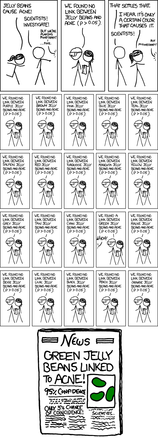
Figure 6:Randall Munroe, xkcd 882 “Significant” (CC BY-NC 2.5) (So, uh, we did the green study again and got no link. It was probably a-- “RESEARCH CONFLICTED ON GREEN JELLY BEAN/ACNE LINK; MORE STUDY RECOMMENDED!”)
To be published in important journals, studies often have to show significant results. That is a problem, because
significant results, too, can be pure accident (the comic),
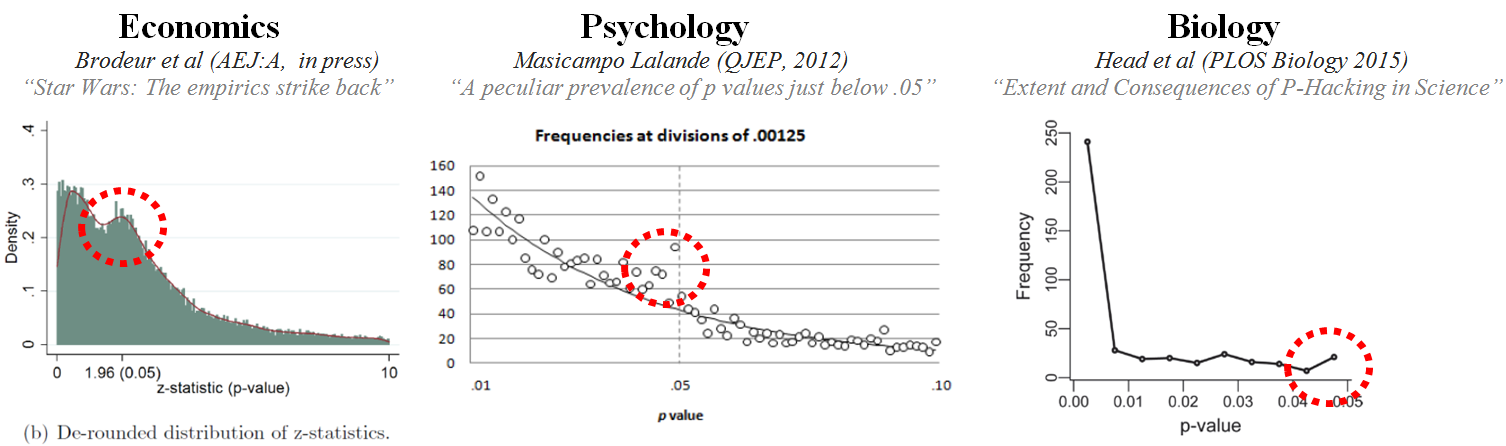
there are tricks for shrinking the p-value systematically without learning anything more about the question (p-value hacking, cf. Figure 7): testing many hypotheses and reporting only the significant one, extending the sample until drops below 0.05, removing outliers after the fact,
non-significant results can be scientifically relevant too, but are published less often (publication bias),
the p-value is very often misread, and not only by students: in the survey of Haller & Krauss (2002), even most of the methodology lecturers got at least one of six statements about the meaning of a significant result wrong.
Most Published Research Findings Are False
Ioannidis JPA (2005) Why Most Published Research Findings Are False. PLOS Medicine 2(8): e124.
“the probability that a research finding is indeed true depends on the prior probability of it being true (before doing the study), the statistical power of the study, and the level of statistical significance”
The less plausible the hypothesis (the lower its prior probability), the more likely an exciting finding is to turn out a false alarm, regardless of the p-value.
A very important safeguard against p-value hacking is the pre-registration of studies: hypothesis, level and analysis are fixed before the data exist. That is exactly what the definition above demands with its “rule fixed in advance”.
What to formulate as hypothesis, what as alternative?
The usual procedure is to formulate the scientific insight you would like to establish as the rejection of the null hypothesis. It makes a difference which statement becomes the hypothesis and which the alternative, because we defined best tests so that the type I and type II errors play different roles: the type I error is held exactly at the level , and the type II error is minimised subject to that constraint.
Even with a type I error can of course still occur, because . The null hypothesis was , where the are the means of the two groups; the alternative is . When we derived the t-test we set up the t-statistic by comparing the sample mean with a fixed . And there the roles of hypothesis and alternative cannot be swapped!
You can see that the two cannot be swapped in the ordinary-language version of the hypothesis too: “the drug has no effect” really means “whether or not you take the drug has no influence on test performance”. How would you formalise “has an influence on test performance” mathematically?
What you can do instead is test for an explicitly described relationship, for example the hypothesis that after taking the drug you score exactly 10 points more in the test – that is, the equation . Note that this is again an equation, whereas cannot be tested in the same way.
Looking ahead: applying further useful tests
There is a whole series of further tests we might need, along with their assumptions and how to run them in Python on a pandas dataset. The applications lie in exploratory data analysis (how is a variable distributed?), in data cleaning (where are the outliers? which variables are so strongly correlated that I keep only one of them?), in data analysis (which statistical dependencies can be modelled?) and in prediction (can I express one variable – the target variable – through the others? that is supervised learning).
Examining one sample
Shapiro–Wilk: : the sample is normally distributed Assumption: the sample is iid
scipy.stats.shapiro
Comparing two samples
Pearson correlation: : the two samples are uncorrelated () Assumption: both samples are iid and jointly normally distributed
scipy.stats.pearsonrChi-squared: : the two samples are independent Assumption: the variable under investigation is categorical, with an expected frequency of at least 5 in every cell of the contingency table
scipy.stats.chi2_contingency
Digression: could a poll have answered the five-per-cent question?
In the German federal election of 23 February 2025 the Bündnis Sahra Wagenknecht won of the second votes (the party vote). It was 9,529 votes (in German) short of entering the Bundestag, out of some 49 million. In the last week before the election twelve polls (in German), each with 1000 to 2500 respondents, had put the BSW between 4 and . Afterwards, the polls were said to have got it wrong. Had they?
Let us check with the recipe. With respondents, a proportion has standard error :
import numpy as np
p = 0.05
for n in [1000, 2000]:
    se = np.sqrt(p * (1 - p) / n)
    print(n, "respondents: standard error", round(100 * se, 2), "points,",
          "95% interval ±", round(196 * se, 2), "points")
1000 respondents: standard error 0.69 points, 95% interval ± 1.35 points
2000 respondents: standard error 0.49 points, 95% interval ± 0.96 pointsSo a poll with 2000 respondents that reports is saying: somewhere between 4 and 6. All twelve polls lay in that range, and so did the election result. None of them “got it wrong”; they answered a question nobody had asked, namely whether the BSW stood at three per cent or at seven. The question people were asking was whether it lay above or below , with a true value of . To resolve two hundredths of a point the interval would have to shrink to points, and because it shrinks only with that would take
almost one in every ten eligible voters. That is no longer a poll, that is an election.
The recipe gives only the lower bound on the uncertainty, the pure sampling error. On top of that comes everything that violates the random-sample assumption: the people who answer the telephone or sit in an online panel are not a random selection of the electorate, so the institutes weight the raw data by age, region and past voting behaviour, each by its own method. Someone who says “BSW” on Tuesday may vote differently on Sunday, or not at all. And the question is “Who would you vote for if there were an election on Sunday?”, not “Who did you vote for?”. The spread from 4 to 6 between the institutes in the same week is partly sampling error and partly these differences of method, and the two can only be told apart once you know how the institute weighted. That is exactly the context without which the number “5%” is not yet a datum.
What this leaves for reading polls is this: a value without an error statement is incomplete; the error statement for 1000 respondents and small parties is about points; and a question whose answer is finer than that interval cannot be answered by any poll, however reputable the institute.
- Allen, M., Babiker, M., Chen, Y., & de Coninck, H. C. (2018). IPCC SR15: Summary for Policymakers. In IPCC Special Report Global Warming of 1.5 oC. Intergovernmental Panel on Climate Change.
- Haller, H., & Krauss, S. (2002). Misinterpretations of Significance: A problem students share with their teachers? Methods of Psychological Research Online, 7(1), 1–20.
- Ioannidis, J. P. A. (2005). Why Most Published Research Findings Are False. PLoS Medicine, 2(8), e124. 10.1371/journal.pmed.0020124