We now have everything we need for an overview of the most important discrete distributions: the pmf from the chapter Random variables and distributions, expected value, variance and entropy from the chapter Expected value and variance, and from the chapter Numpy the machinery for actually computing with them.
We present every distribution in the same format – parameters, pmf, expected value, variance,
entropy, example applications and the name in scipy.stats – just as we will later do for the
continuous distributions.
Convention: discrete probability spaces
In this chapter is always at most countable, and usually even finite. Then the power set is a σ-algebra, so every subset of is an event, and the probability measure is completely determined by the values
on the individual outcomes – because every event is the (at most countable) disjoint union of its elements, so that . This function is the probability mass function (pmf); discrete density is another name in common use. Everything we want to know about a discrete distribution can be read off it:
Discrete distributions in SciPy
scipy.stats provides objects for discrete distributions just as it does for continuous ones.
The main difference: where a continuous distribution has a density pdf, a discrete
distribution has a pmf, and the method is accordingly called pmf.
import numpy as np
import matplotlib.pyplot as plt
import scipy.stats as st


def plotXdiscrete(k, X, name, params):
    description = ", ".join(f"{value}" for value in params)
    fig, axs = plt.subplots(1, 2, figsize=(12, 4))
    # First the probability mass function:
    axs[0].stem(k, X.pmf(k), basefmt=" ")
    axs[0].set_xlabel("$k$")
    axs[0].set_ylabel("$p(k) = P(X = k)$")
    axs[0].set_title(f"pmf of the {name} with {description}")
    # Then the cumulative distribution function:
    axs[1].step(k, X.cdf(k), where="post")
    axs[1].set_xlabel("$k$")
    axs[1].set_ylabel("$F(k) = P(X \\leq k)$")
    axs[1].set_title(f"cdf of the {name}")
    # tight_layout keeps the two sets of axis labels from overlapping:
    plt.tight_layout()
    plt.show()
The methods we need over and over again are the same for every distribution.
If X is a discrete random variable from scipy.stats, then:
| wanted | call |
|---|---|
X.pmf(k) | |
X.cdf(k) | |
X.sf(k), equivalent to 1 - X.cdf(k) | |
X.sf(k-1) | |
X.cdf(k-1) | |
| a sample of size | X.rvs(size=n) |
| , , | X.mean(), X.var(), X.std() |
The sf stands for survival function.
X = st.binom(10, 0.3)
print("P(X = 3)   =", X.pmf(3))
print("P(X <= 3)  =", X.cdf(3))
print("P(X > 3)   =", X.sf(3), "= 1 - P(X <= 3) =", 1 - X.cdf(3))
print("P(X >= 3)  =", X.sf(2))
assert np.isclose(X.cdf(3) + X.sf(3), 1.0)
P(X = 3)   = 0.2668279319999998
P(X <= 3)  = 0.6496107184000002
P(X > 3)   = 0.3503892815999998 = 1 - P(X <= 3) = 0.3503892815999998
P(X >= 3)  = 0.6172172136000003
Discrete uniform distribution
Parameter , notation
pmf for
Expected value
Variance
Entropy – the maximum among all distributions on a set with elements (see Expected value and variance, section Entropy)
Example applications:
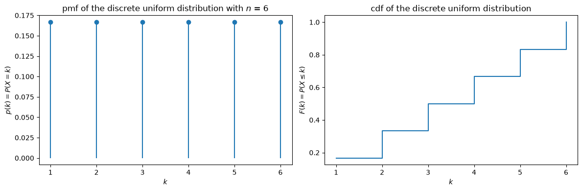
The fair die: , so and .
An idealised random number generator that returns integers in a fixed range.
In
scipy.stats:st.randint(1, n+1)– careful: as withrange, the upper bound is exclusive.
We already know the expected value. For the variance we use . With the summation formula we get
and therefore
n = 6
X = st.randint(1, n + 1)   # upper bound exclusive, so 1 to 6
print("E(X) =", X.mean(), " expected:", (n + 1) / 2)
print("V(X) =", X.var(),  " expected:", (n**2 - 1) / 12)

plotXdiscrete(np.arange(1, n + 1), X, "discrete uniform distribution", (f"$n$ = {n}",))
E(X) = 3.5  expected: 3.5
V(X) = 2.9166666666666665  expected: 2.9166666666666665
Categorical distribution
Parameter a probability vector , that is and
pmf on a set with elements
Expected value (if we identify with the number ) – which in general does not simplify any further
Variance
Entropy
Example applications:
An urn with balls in colours, of them of colour ; drawing with replacement gives .
Any survey with a fixed list of mutually exclusive answers.
In
scipy.stats: no object of its own, butst.rv_discrete(values=(values, p))builds one; if all you want is to draw samples,rng.choice(values, p=p)from the chapter Numpy is enough.
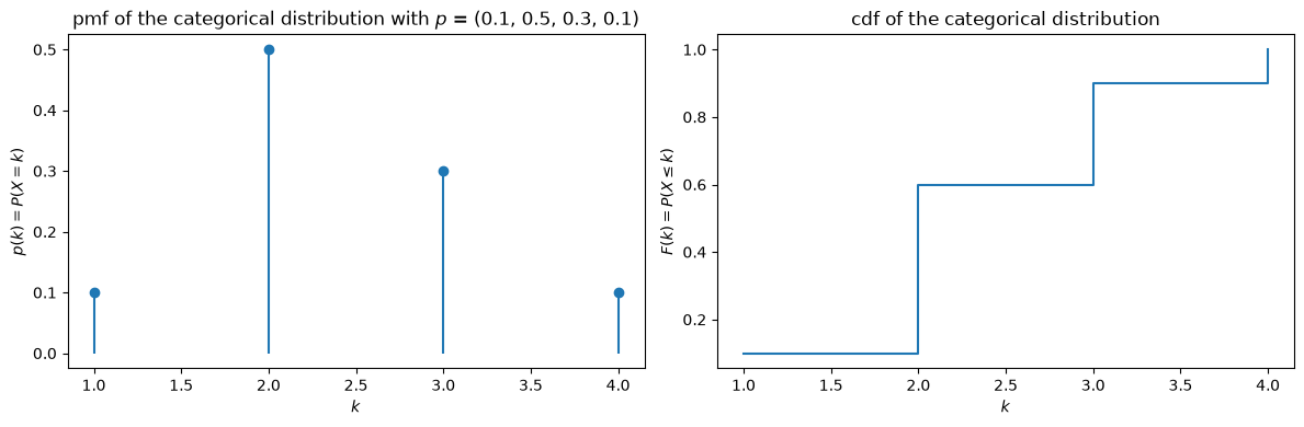
The parameter space is exactly the simplex we met in the chapter Random variables and distributions: the uniform distribution sits at its centre, the Dirac distributions at its vertices. The categorical distribution is therefore the most general distribution on a finite set – every distribution that follows in this chapter is either a special case of it or built from it. The four jumper colours from that chapter are a categorical distribution too, with .
values = np.arange(1, 5)
p = np.array([0.1, 0.5, 0.3, 0.1])
X = st.rv_discrete(values=(values, p))

print("E(X) =", X.mean(), " recomputed:", np.sum(values * p))
print("V(X) =", X.var())
print("H(X) =", X.entropy() / np.log(2), "bits")   # scipy computes in nats
print("for comparison, uniform distribution on 4 values:", np.log2(4), "bits")

plotXdiscrete(values, X, "categorical distribution", (f"$p$ = {tuple(p.tolist())}",))
E(X) = 2.4  recomputed: 2.4
V(X) = 0.6400000000000006
H(X) = 1.6854752972273344 bits
for comparison, uniform distribution on 4 values: 2.0 bits
Bernoulli distribution
Parameter , notation
pmf and on
Expected value
Variance
Entropy , the binary entropy function
Example applications:
A single coin toss, unfair coins included.
Any yes/no feature: a component is defective or it is not, an email is spam or it is not.
In
scipy.stats:st.bernoulli(p)
The Bernoulli distribution is the special case of the categorical distribution, and the simplest nontrivial case there is – it has one parameter. Expected value and variance are quick to compute: , and since (because and ), we also have and therefore
The variance is maximal at and vanishes for – there the outcome is no longer random at all.
In the chapter Random variables and distributions we already estimated a value from data without giving it a name: it was the parameter of a Bernoulli distribution.
The binary entropy function
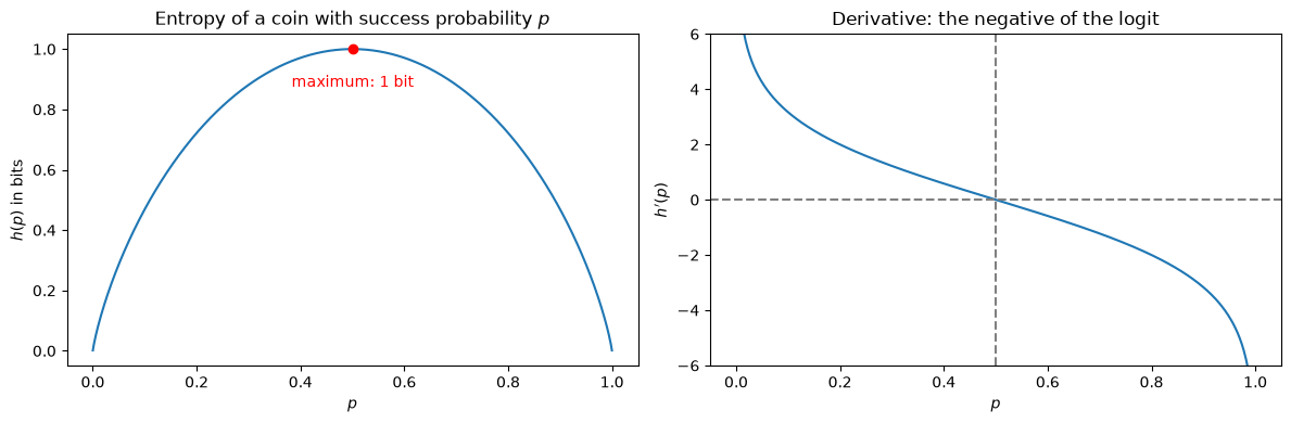
The entropy of a Bernoulli distribution, as a function of , deserves a look of its own. Let us differentiate it. With we have
so the two constants cancel and what remains is
The only zero is at , that is, at : the fair coin toss has the maximal entropy, namely bit. That fits: the uniform distribution is the maximum entropy distribution.
p = np.linspace(1e-4, 1 - 1e-4, 500)
h = -p * np.log2(p) - (1 - p) * np.log2(1 - p)
h_prime = -np.log2(p / (1 - p))

fig, axs = plt.subplots(1, 2, figsize=(12, 4))

axs[0].plot(p, h)
axs[0].plot(0.5, 1.0, "o", color="red")
axs[0].annotate("maximum: 1 bit", (0.5, 1.0), textcoords="offset points",
                xytext=(0, -25), ha="center", color="red")
axs[0].set_xlabel("$p$")
axs[0].set_ylabel("$h(p)$ in bits")
axs[0].set_title("Entropy of a coin with success probability $p$")

axs[1].plot(p, h_prime)
axs[1].axhline(0, linestyle="--", color="gray")
axs[1].axvline(0.5, linestyle="--", color="gray")
axs[1].set_ylim(-6, 6)
axs[1].set_xlabel("$p$")
axs[1].set_ylabel("$h'(p)$")
axs[1].set_title("Derivative: the negative of the logit")

plt.tight_layout()
plt.show()

X = st.bernoulli(0.3)
print("E(X) =", X.mean(), " V(X) =", X.var(), " H(X) =", X.entropy() / np.log(2), "bits")
E(X) = 0.3 V(X) = 0.21 H(X) = 0.8812908992306927 bits
Binomial distribution
Parameters and , notation
pmf for
Expected value
Variance
Entropy: no convenient closed expression; it is smaller than , since the maximum would be the uniform distribution on
Example applications:
Tossing the same coin times and counting the heads.
Drawing a sample of components and counting the defective ones.
An urn with two colours, balls of which are red, , drawing times with replacement.
In
scipy.stats:st.binom(n, p)
The binomial distribution arises from the Bernoulli distribution by repetition. If are independent random variables with , then
counts the number of successes, and . So it has two parameters.
Why the pmf looks the way it does: by independence, any one fixed pattern of successes and failures – say – has probability , whichever positions the successes occupy. And there are exactly such patterns, one for each subset of with elements. Summing over them gives the formula.
Expected value and variance now come for free. The expected value follows from linearity:
For the variance we need the independence – this is exactly the rule of calculation from the section Rules of calculation for the variance:
Without independence this would be false. Here you can see clearly what that rule is good for.
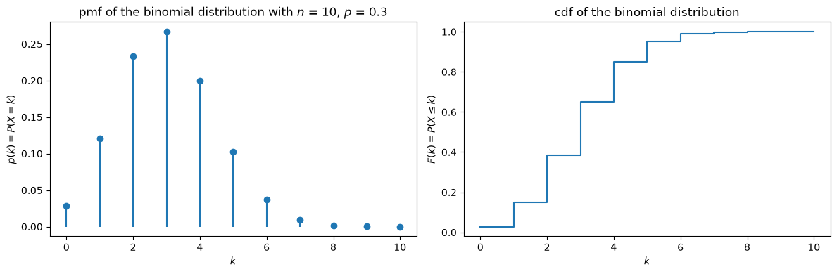
n, p = 10, 0.3
X = st.binom(n, p)
print("E(X) =", X.mean(), " expected:", n * p)
print("V(X) =", X.var(),  " expected:", n * p * (1 - p))

plotXdiscrete(np.arange(0, n + 1), X, "binomial distribution", (f"$n$ = {n}", f"$p$ = {p}"))
E(X) = 3.0  expected: 3.0
V(X) = 2.1  expected: 2.0999999999999996
Which fits the data best?
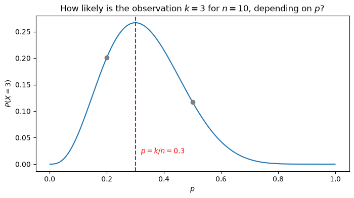
So far we have treated as given and asked for the probability of successes. Now we turn the question around: we have found defective components in a sample of and want to know which fits this observation.
For every the pmf gives us a probability for exactly this observation:
Let us compare two candidates, and . The binomial coefficient is the same in both cases and cancels, so it is enough to compare :
So our observation is about 1.7 times as likely under as under . In this sense fits better.
The natural next question is which fits best of all. We are looking for the maximum of , so we differentiate:
For the leading factor is nonzero, so what remains is the condition . Solving it: , so and therefore
For our observation that is – simply the proportion of successes in the sample. That is exactly what you would have guessed without any calculation; what is remarkable is that here it drops out of a calculation, from a clearly stated criterion: choose the parameter that makes the observation you actually made as likely as possible.
k, n = 3, 10
p = np.linspace(0.001, 0.999, 500)
probability = st.binom(n, p).pmf(k)

fig, ax = plt.subplots(figsize=(8, 4))
ax.plot(p, probability)
ax.axvline(k / n, linestyle="--", color="red")
ax.annotate(f"$p = k/n = {k/n}$", (k / n, 0.02), color="red",
            textcoords="offset points", xytext=(8, 0))
for candidate in (0.2, 0.5):
    ax.plot(candidate, st.binom(n, candidate).pmf(k), "o", color="gray")
ax.set_xlabel("$p$")
ax.set_ylabel(f"$P(X = {k})$")
ax.set_title(f"How likely is the observation $k={k}$ for $n={n}$, depending on $p$?")
plt.show()

print("P(X=3) at p=0.2:", st.binom(n, 0.2).pmf(k))
print("P(X=3) at p=0.5:", st.binom(n, 0.5).pmf(k))
print("P(X=3) at p=0.3:", st.binom(n, 0.3).pmf(k), "  <- the maximum")
P(X=3) at p=0.2: 0.20132659199999992
P(X=3) at p=0.5: 0.1171875
P(X=3) at p=0.3: 0.2668279319999998   <- the maximum
This procedure – choosing the parameter that makes the observation most likely – is called maximum likelihood estimation. The chapter Statistical models treats it in general and for other distributions.
Digression: the Poisson binomial distribution
Parameters , one probability per trial
pmf , where is the set of subsets of with elements
Expected value
Variance
Example application: components from different batches, each with its own failure probability – how many of them fail?
In
scipy.stats: no object of its own; the pmf is easy enough to compute yourself.
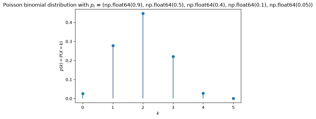
We are no longer tossing the same coin times but different coins, each with its own success probability . The are still independent, just no longer identically distributed. Expected value and variance therefore follow exactly as for the binomial distribution, from linearity and from the variance rule for independent summands; when all the are equal, as for the binomial distribution, we get and back.
The pmf itself is unwieldy – the sum runs over subsets. In practice it is computed iteratively: start with “no coins, no successes, with probability 1” and work the coins in one at a time.
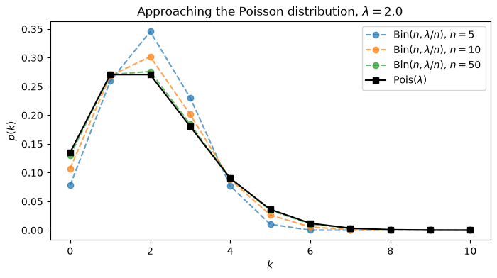
The interesting case is many small . If we set every and let grow, the expected value stays fixed at while each individual trial becomes ever less likely. This is the passage to the Poisson distribution:
def poisson_binomial_pmf(ps):
    """pmf of a Poisson binomial distribution, built up iteratively.

    We start with "no coins, no successes" and work the coins in one at a time:
    distribution[k] is the probability of k successes among the coins considered so far.
    """
    distribution = np.array([1.0])
    for p in ps:
        without_success = np.append(distribution * (1 - p), 0.0)
        with_success = np.append(0.0, distribution * p)
        distribution = without_success + with_success
    return distribution


ps = np.array([0.9, 0.5, 0.4, 0.1, 0.05])
pmf = poisson_binomial_pmf(ps)
k = np.arange(len(pmf))

print("sum of the pmf =", pmf.sum())
print("E(X) =", np.sum(k * pmf), " expected:", ps.sum())
print("V(X) =", np.sum(k**2 * pmf) - np.sum(k * pmf) ** 2, " expected:", np.sum(ps * (1 - ps)))

fig, ax = plt.subplots(figsize=(7, 4))
ax.stem(k, pmf, basefmt=" ")
ax.set_xlabel("$k$")
ax.set_ylabel("$p(k) = P(X = k)$")
ax.set_title(f"Poisson binomial distribution with $p_i$ = {tuple(ps)}")
plt.show()
sum of the pmf = 1.0
E(X) = 1.9500000000000004  expected: 1.95
V(X) = 0.7174999999999998  expected: 0.7174999999999999
# The passage to the limit: all p_i equal to lambda/n, n grows.
lam = 2.0
k = np.arange(0, 11)

fig, ax = plt.subplots(figsize=(8, 4))
for n in (5, 10, 50):
    ax.plot(k, st.binom(n, lam / n).pmf(k), "o--", alpha=0.7, label=f"$\\operatorname{{Bin}}(n, \\lambda/n)$, $n={n}$")
ax.plot(k, st.poisson(lam).pmf(k), "s-", color="black", label="$\\operatorname{Pois}(\\lambda)$")
ax.set_xlabel("$k$")
ax.set_ylabel("$p(k)$")
ax.set_title(f"Approaching the Poisson distribution, $\\lambda = {lam}$")
ax.legend()
plt.show()
Poisson distribution
Parameter , notation
pmf for
Expected value
Variance
Example applications:
How many requests reach the server in one second?
How many typos are there on one page?
How many atomic nuclei in a specimen decay in one minute?
In
scipy.stats:st.poisson(mu=λ)
The guiding question: how many events occur in a fixed period of time, if they occur independently of one another and at a constant mean rate? In contrast to every distribution in this chapter so far, this one does not have finite support – in principle there could be arbitrarily many events, even if large numbers become very unlikely.
That the pmf sums to 1 follows from the exponential series :
The expected value follows with an index shift – the summand for is 0 and drops out:
For the variance, compute in just the same way, which gives . So here expected value and variance coincide – a practical test of whether a Poisson distribution can fit a dataset at all.
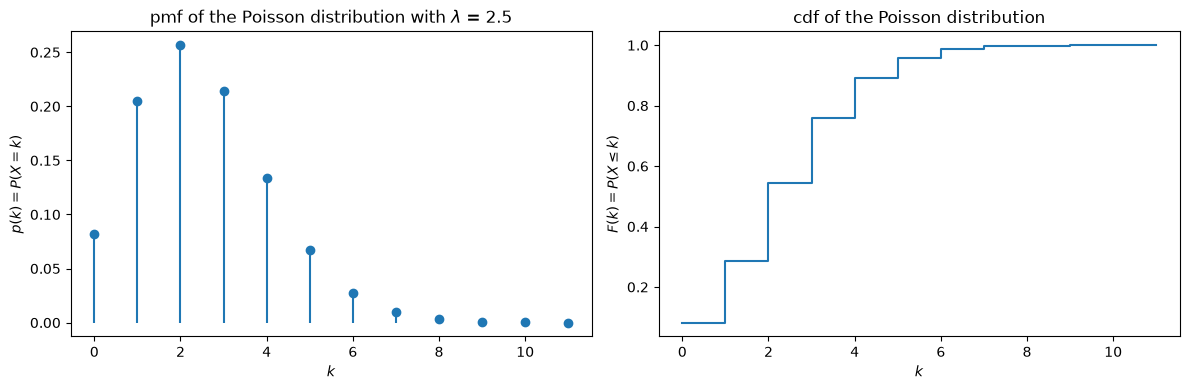
lam = 2.5
X = st.poisson(lam)
print("E(X) =", X.mean(), " V(X) =", X.var(), " (both equal to lambda)")
print("P(X > 2) =", X.sf(2), " by hand:", 1 - np.exp(-lam) * (1 + lam + lam**2 / 2))

plotXdiscrete(np.arange(0, 12), X, "Poisson distribution", (f"$\\lambda$ = {lam}",))
E(X) = 2.5  V(X) = 2.5  (both equal to lambda)
P(X > 2) = 0.45618688411667035  by hand: 0.4561868841166704
For completeness: the geometric distribution
Parameter , notation
pmf for
Expected value
Variance
Example applications:
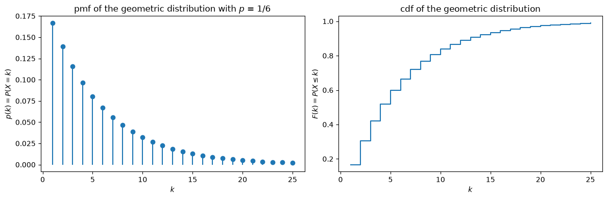
How many times do I have to throw a die until the first six comes up? (, on average 6 throws)
How many connection attempts does it take until the first success?
In
scipy.stats:st.geom(p)
We repeat a Bernoulli experiment until the first success and count the trials. For the first trials to fail and the -th to succeed has probability – hence the pmf.
The geometric distribution is memoryless: if you have already thrown the die ten times in vain, the probability of needing another throws is the same as it was at the start. The die does not remember. It is thus the discrete counterpart of the exponential distribution, the only memoryless distribution in the continuous case.
p = 1 / 6
X = st.geom(p)
print("E(X) =", X.mean(), " expected:", 1 / p)
print("V(X) =", X.var(),  " expected:", (1 - p) / p**2)

plotXdiscrete(np.arange(1, 26), X, "geometric distribution", (f"$p$ = 1/6",))
E(X) = 6.0  expected: 6.0
V(X) = 30.000000000000007  expected: 30.000000000000004
Looking back
All the distributions in this chapter hang together:
The categorical distribution is the most general distribution on a finite set; its parameter space is the simplex .
The discrete uniform distribution is the centre of that simplex and has maximal entropy.
The Bernoulli distribution is the case .
The binomial distribution counts the successes in independent Bernoulli trials with the same , the Poisson binomial distribution allows different .
The Poisson distribution is their limiting case for many trials, each of them very unlikely.
The geometric distribution turns the question around: not how many successes in a fixed number of trials, but how many trials up to the first success.
Next we leave countable sets of outcomes behind. Look at the binomial distribution not for small but for large , and the passage to the limit leads not to the Poisson distribution but to the normal distribution – that is the de Moivre–Laplace theorem, and the chapter The normal distribution opens with it.