The first chapter said that most of a data scientist’s working day goes not on modelling but on obtaining data, cleaning it and communicating results. This chapter is about the cleaning – “data scrubbing”: spotting outliers, handling missing values, repairing data types, taking text apart with regular expressions, reading dates and times correctly. None of it is mathematically deep, and all of it decides whether the models of the chapters that follow are any good.
The example data are daily values from the Düsseldorf weather station, taken from the open data portal of the German weather service (DWD), and, at the end, the Titanic dataset for the text processing.
Loading the data and a first look
For each station the DWD supplies a ZIP archive containing one data file and several metadata files. Missing values are coded as -999 – a fact stated in the file’s description, not in the file itself. Without that piece of information Pandas would read -999 as a valid temperature, and the mean would be nonsense.
import numpy as np
import pandas as pd
import matplotlib.pyplot as plt
import zipfile, urllib.request, pathlib

base = "https://opendata.dwd.de/climate_environment/CDC/observations_germany/climate/daily/kl/historical/"
station = "01078"                                    # Düsseldorf
folder = pathlib.Path(base.replace("https://", ""))  # local copy, same path as on the web

# The file name contains the end date and changes every year, as soon as the DWD appends
# another year. So we search for it: locally first, otherwise in the server's directory listing.
local = sorted(folder.glob(f"tageswerte_KL_{station}_*_hist.zip"))
if local:
    path = local[-1]
else:
    import re
    listing = urllib.request.urlopen(base).read().decode("utf-8")
    filename = re.search(rf"tageswerte_KL_{station}_\d{{8}}_\d{{8}}_hist\.zip", listing).group(0)
    path = folder / filename
    folder.mkdir(parents=True, exist_ok=True)
    urllib.request.urlretrieve(base + path.name, path)

with zipfile.ZipFile(path) as archive:
    data_file = [name for name in archive.namelist() if name.startswith("produkt_klima_tag")][0]
    raw = pd.read_csv(archive.open(data_file), sep=";", skipinitialspace=True, na_values=-999)

raw.columns = raw.columns.str.strip()                   # column names have leading spaces
raw = raw.drop(columns="eor")                           # "end of record", no content
print(raw.shape)
raw.tail(3)
(27029, 18)
The column names are shorthand codes explained in the metadata file: TMK is the daily mean temperature, TXK and TNK the maximum and the minimum, RSK the amount of precipitation in mm, SDK the duration of sunshine in hours, PM the air pressure, UPM the relative humidity. We keep the columns we need, give them telling names and restrict ourselves to 2025. The date stays an integer of the form YYYYMMDD for now; the section on date and time deals with it.
weather = (raw.rename(columns={"MESS_DATUM": "date_raw", "TMK": "temp_mean", "TXK": "temp_max",
                               "TNK": "temp_min", "RSK": "precipitation", "SDK": "sunshine", "PM": "pressure", "UPM": "humidity"})
              .loc[:, ["date_raw", "temp_mean", "temp_max", "temp_min", "precipitation", "sunshine", "pressure", "humidity"]])
weather = weather[(weather["date_raw"] >= 20250101) & (weather["date_raw"] <= 20251231)].reset_index(drop=True)
weather.info()
print("\nMissing values per column:")
print(weather.isna().sum())
<class 'pandas.DataFrame'>
RangeIndex: 365 entries, 0 to 364
Data columns (total 8 columns):
# Column Non-Null Count Dtype
--- ------ -------------- -----
0 date_raw 365 non-null int64
1 temp_mean 365 non-null float64
2 temp_max 365 non-null float64
3 temp_min 365 non-null float64
4 precipitation 364 non-null float64
5 sunshine 21 non-null float64
6 pressure 355 non-null float64
7 humidity 346 non-null float64
dtypes: float64(7), int64(1)
memory usage: 22.9 KB
Missing values per column:
date_raw 0
temp_mean 0
temp_max 0
temp_min 0
precipitation 1
sunshine 344
pressure 10
humidity 19
dtype: int64
The duration of sunshine is missing on almost every day of 2025; air pressure and humidity have the odd gap. The data file does not say why; the answer is in the archive’s metadata files, which is exactly why those have to be read too. These are genuine gaps, of the kind every dataset has. To assess how gaps are handled, though, we need gaps whose true value we know. So we make a copy and deliberately delete a random 10% of its daily mean temperatures. That is rule 3 in action: only with a known truth can we measure which repair is best.
rng = np.random.default_rng(2025)
truth = weather["temp_mean"].copy()
deleted = rng.random(len(weather)) < 0.10              # mask: which values we "lose"
broken = weather.copy()
broken.loc[deleted, "temp_mean"] = np.nan
broken["temp_mean_missing"] = deleted                  # rule 1: the change is logged as a column
print(f"{deleted.sum()} of {len(weather)} daily means removed")
30 of 365 daily means removed
Outliers
An outlier is a value so far from the others that it is either a measurement error or a rare event that skews the picture. The number itself will not tell you which; that has to be decided from the context. The first step is always to look. To have something to look at, we build in two errors typical of transcribed measurements: a temperature without its decimal point, and a sign error.
faulty = broken.copy()
faulty.loc[150, "temp_mean"] = 231.0     # 23.1 typed without the decimal point
faulty.loc[300, "temp_mean"] = -45.0     # sign and digit transposed

fig, axs = plt.subplots(1, 2, figsize=(12, 3.5))
axs[0].plot(faulty["temp_mean"].values); axs[0].set_title("Daily mean temperature, with errors")
axs[1].hist(faulty["temp_mean"].dropna(), bins=60); axs[1].set_title("Histogram")
plt.show()
print("Mean with errors:", faulty["temp_mean"].mean().round(2),
      " without errors:", broken["temp_mean"].mean().round(2))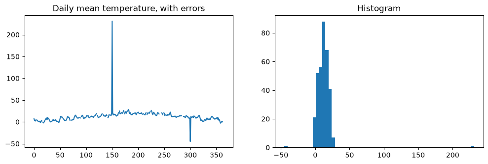
Mean with errors: 12.21 without errors: 11.75
In the plot both errors are obvious at once; in the mean they hide behind half a degree. The systematic way to find such values is the z-score, the deviation from the mean in units of the standard deviation (see Expected value and variance). The usual rule of thumb: values with count as outliers. Under a normal distribution only one value in 370 lies that far out.
column = faulty["temp_mean"]
z = (column - column.mean()) / column.std(ddof=0)      # z-score by hand; NaN stay NaN, scipy.stats.zscore would do too
outliers = z.abs() > 3                                 # careful: "< 3" would be the mask of the *non*-outliers; NaN gives False
print(faulty.loc[outliers, ["date_raw", "temp_mean"]])
     date_raw  temp_mean
150  20250531      231.0
300  20251028      -45.0
Both errors we built in are found, and nothing else is. That is not a given: the z-score relies on the mean and the standard deviation, and the outliers themselves distort both. A single very large error can inflate the standard deviation so much that smaller errors stay below the threshold. The variant built on the median and the interquartile range, the one the boxplot uses, is more robust.
What do you do with an outlier once you have found it? Not delete the row: the other columns for that day are fine. Set the value to NaN instead, so that the next section treats it like any other missing value, and keep the mask.
cleaned = faulty.copy()
cleaned["temp_mean_outlier"] = outliers
cleaned.loc[outliers, "temp_mean"] = np.nan
print("Mean after cleaning:", cleaned["temp_mean"].mean().round(2))
Mean after cleaning: 11.73
Missing values
Pandas has three answers to a missing value: ignore it (most summary measures, mean among them, simply leave NaN out), discard the row (dropna), or insert a substitute value (fillna, imputation). Discarding is honest but costs data, and not at random: if the duration of sunshine is missing for precisely the last few months, dropna throws away precisely those months. Imputation keeps the rows but invents values, and the question is which substitute values do the least damage. We compare the usual strategies on the daily mean temperatures we deleted on purpose, where we know the truth, with the mean absolute error as the target metric.
column = cleaned["temp_mean"]
month = cleaned["date_raw"] // 100 % 100                     # month number out of YYYYMMDD

strategies = {
    "constant 0":            column.fillna(0),
    "global mean":           column.fillna(column.mean()),
    "global median":         column.fillna(column.median()),
    "monthly mean":          column.fillna(column.groupby(month).transform("mean")),
    "last value (ffill)":    column.ffill(),
    "linear interpolation":  column.interpolate(),
}
result = {name: (replacement[deleted] - truth[deleted]).abs().mean() for name, replacement in strategies.items()}
pd.Series(result, name="MAE in °C").round(2).sort_values()
linear interpolation 1.28
last value (ffill) 1.60
monthly mean 2.90
global median 6.11
global mean 6.23
constant 0 13.92
Name: MAE in °C, dtype: float64The ranking is typical of time series: whatever knows the neighbours (interpolation, last value) beats whatever knows only the group (monthly mean), which in turn beats whatever knows only the whole (global mean or median). The constant 0 trails far behind and is nevertheless common in practice, because some tools use it as their default. For other data the ranking can look different: for a column with no temporal order ffill is pointless, and for skewed distributions with outliers the median is preferable to the mean.
Two details that come up again and again:
groupby(...).transform("mean")computes the mean of each group and writes it back into every row of that group; the result is as long as the column and can go straight intofillna. If a group is entirely empty, its mean isNaNand the gap stays a gap – as it should.Older guides write
fillna(method="ffill"). That no longer exists in Pandas 3; the methods are nowffill()andbfill().
And rule 1 once more: after imputation the column itself no longer knows which of its values are real. The mask temp_mean_missing from the start is the only place where that information survives.
cleaned["temp_mean"] = cleaned["temp_mean"].interpolate()
cleaned["temp_mean_imputed"] = cleaned["temp_mean_missing"] | cleaned["temp_mean_outlier"]
print(cleaned["temp_mean_imputed"].sum(), "values in the column are not measured but inserted")
32 values in the column are not measured but inserted
Data types, encoding and categorical values
The first check after loading is info(): if a column of numbers has type object, some text has crept in – a comma as decimal separator, say, a k.A. (“no information”) or a thousands separator. Such a column is repaired with pd.to_numeric(..., errors="coerce"), which turns everything unreadable into NaN; afterwards you count how many values that affected.
Text also has an encoding. A file is a sequence of bytes, and only the encoding says which bytes stand for which character. The standard is UTF-8; older files from Windows programs are often in Latin-1 or Windows-1252. Assume the wrong encoding and you get either an error message or, worse, silently wrong characters.
word = "Düsseldorf"
utf8 = word.encode("utf-8")
latin1 = word.encode("latin-1")
print("UTF-8:  ", utf8, len(utf8), "bytes")
print("Latin-1:", latin1, len(latin1), "bytes")
print("Latin-1 bytes read as UTF-8:", latin1.decode("utf-8", errors="replace"))
print("UTF-8 bytes read as Latin-1:", utf8.decode("latin-1"))
UTF-8: b'D\xc3\xbcsseldorf' 11 bytes
Latin-1: b'D\xfcsseldorf' 10 bytes
Latin-1 bytes read as UTF-8: D�sseldorf
UTF-8 bytes read as Latin-1: Düsseldorf
The second result is the notorious Düsseldorf that haunts so many databases: somebody read UTF-8 as Latin-1 and saved the result. pd.read_csv has an encoding parameter for this; when in doubt, look at the first few bytes of the file with open(..., "rb").
Categorical values from free-text fields arrive in many spellings. The route is always the same: normalise first (strip spaces, lower-case), then merge the remaining variants with a mapping table, and catch typos by string similarity. The standard library ships difflib for that; if you need something more exact, use the edit distance (Levenshtein distance), the number of insertions, deletions and substitutions between two strings.
import difflib

city = pd.Series(["Düsseldorf", "Duesseldorf", "düsseldorf ", "Dusseldorf", "Köln", "Koeln", "Düsseldorf", "Kln"])
normalised = city.str.strip().str.lower().str.replace("ue", "ü").str.replace("oe", "ö")
table = {"dusseldorf": "düsseldorf"}                         # known variants spelled out
normalised = normalised.replace(table)
known = ["düsseldorf", "köln"]
def closest(s):
    matches = difflib.get_close_matches(s, known, n=1, cutoff=0.6)
    return matches[0] if matches else s
result = normalised.map(closest)
print(pd.DataFrame({"raw": city, "normalised": normalised, "assigned": result}))
print("\nDistinct values before:", city.nunique(), " after:", result.nunique())
raw normalised assigned
0 Düsseldorf düsseldorf düsseldorf
1 Duesseldorf düsseldorf düsseldorf
2 düsseldorf düsseldorf düsseldorf
3 Dusseldorf düsseldorf düsseldorf
4 Köln köln köln
5 Koeln köln köln
6 Düsseldorf düsseldorf düsseldorf
7 Kln kln köln
Distinct values before: 7 after: 2
Seven spellings become two cities. This too is a distortion: assigning Kln to köln is a guess, and if a city called “Kln” really existed it would be wrong. That is why the table of assignments belongs in the log.
How categorical values are then turned into numbers (ordinal and one-hot encoding) is covered by the table of levels of measurement in the chapter Descriptive statistics.
Regular expressions
As soon as a column contains text you want to pull something out of (the title from a name, the domain from a URL, the postcode from an address), you need regular expressions. Their reputation as cryptic strings of symbols comes from the notation, not from the thing itself. A regular expression is a compact description of a finite automaton, of the kind you know from the course on formal languages: it runs over the string from left to right and decides at each position whether the character fits. Two rules make working with them bearable:
Write regular expressions across several lines, with comments. Python allows this with the flag
re.VERBOSE: spaces and line breaks in the pattern are then ignored, and anything after a#is a comment.Put whatever you want to pull out in groups.
re.searchreturns the groups, and Pandas’str.extractturns them into columns.
import re

urls = pd.Series(["https://www.hhu.de/studium", "http://opendata.dwd.de/climate_environment/CDC/",
                  "https://voelkel.pages.cs.uni-duesseldorf.de/ds-skript/", "mailto:info@example.org"])
pattern = re.compile(r"""
    ^https?://          # scheme: http or https, then ://
    ([^/]+)             # group 1: everything up to the next slash, that is the host
    (/.*)?$             # group 2 (optional): the path from the slash onwards
""", re.VERBOSE)
print(urls.str.extract(pattern))
0 1
0 www.hhu.de /studium
1 opendata.dwd.de /climate_environment/CDC/
2 voelkel.pages.cs.uni-duesseldorf.de /ds-skript/
3 NaN NaN
The last row is NaN, because mailto: does not fit the pattern. That is intended: a regular expression tells you not only what it finds but also that something fails to conform to the expected format. The number of NaNs after an extract is therefore a measure of data quality.
The commonest trap is the greed of the repetition operators. .* grabs as many characters as it can and gives back only as many as the rest of the pattern needs in order to fit. For the automaton that means running to the end and then backing up. The “lazy” variant .*? takes as little as possible.
html = '<a href="one.html">One</a> and <a href="two.html">Two</a>'
print("greedy:", re.findall(r'<a href="(.*)">', html))     # takes up to the last ">
print("lazy:  ", re.findall(r'<a href="(.*?)">', html))    # takes up to the next ">
greedy: ['one.html">One</a> and <a href="two.html']
lazy: ['one.html', 'two.html']
Two constructions are worth learning, because they solve problems you could otherwise tinker with for a long time.
The negative lookahead (?!…) checks that something is not at this position, without consuming any characters in the process. So (?!23)\d\d matches every two-digit number except 23. Its counterpart (?=…) demands that something does follow.
A backreference \1 stands for whatever group 1 matched, and demands that exactly the same thing appear once more. That is how you find doubled words – the classic typo that the spell checkers of early word processors never caught.
print(re.findall(r"(?!23)\d\d", "22 23 24"))   # 23 is missing, 22 and 24 are there

doubled = re.compile(r"\b(\w+)\s+\1\b")
print(doubled.search("She is the the best")[1])        # 'the'
print(doubled.sub(r"\1", "She is the the best"))       # once is enough
['22', '24']
the
She is the best
Groups are also why a pattern can return more than “matches / does not match”. The pattern
r"^<([a-z]+?)>(.*)</([a-z]+?)>$"takes "<p>html code</p>" apart into the three groups "p", "html code" and "p". But it also shows the limit straight away: it does not match '<a href="url">text</a>', because the opening tag has an attribute in it. You can extend the pattern, and then comes the next counterexample. The lesson from this is well known and still holds unchanged: you do not take HTML apart with regular expressions but with a parser – HTML is not a regular language, and no finite automaton can count nested tags. For a single, known field in a text column, on the other hand, regular expressions are exactly the right tool.
You rarely need more than these building blocks. The following table is the short version, read from the top (binding weakly) to the bottom (binding strongly):
| Building block | Notation | Example | Matches |
|---|---|---|---|
| alternation | A|B | a|b | a or b |
| concatenation | AB | ab | ab |
| repetition, any number of times | A* | a* | nothing, a, aa, … |
| repetition, at least once | A+ | a+ | a, aa, … |
| repetition, optional | A? | a? | nothing or a |
| repetition, counted | A{n,m} | a{2,4} | aa, aaa, aaaa |
| group | (A) | (ab|c) | ab or c, and remembered as a group |
| any character | . | ab.d | abcd, ab7d, … |
| character class | […] | [abc], [a-z] | one of the characters named |
| negated character class | [^…] | [^def] | anything except d, e, f |
| anchor | ^, $ | abc$ | abc at the end of the line |
Characters with a special meaning (., *, +, ?, (, ), [, ], |, ^, $, \) get a backslash in front of them when they are meant literally: \. matches a full stop. That is why patterns in Python are always written as a raw string r"…" – otherwise every backslash would have to be doubled.
If you work with them regularly, read Friedl’s book at some point Friedl (2006); it explains how the automata really run and why some patterns are slow.
Notebook Cell
titanic = pd.read_csv("titanic.csv")
titanic["Title"] = titanic["Name"].str.extract(r",\s*([^.]+)\.")    # after the comma up to the first full stop
print(titanic["Title"].value_counts())
Title
Mr 517
Miss 182
Mrs 125
Master 40
Dr 7
Rev 6
Major 2
Mlle 2
Col 2
Don 1
Mme 1
Ms 1
Lady 1
Sir 1
Capt 1
the Countess 1
Jonkheer 1
Name: count, dtype: int64
Notebook Cell
combine = {"Mlle": "Miss", "Ms": "Miss", "Mme": "Mrs",
           "Dr": "Rank", "Rev": "Rank", "Col": "Rank", "Major": "Rank", "Capt": "Rank",
           "Sir": "Nobility", "Lady": "Nobility", "the Countess": "Nobility", "Don": "Nobility", "Jonkheer": "Nobility"}
titanic["Title"] = titanic["Title"].replace(combine)
titanic.groupby("Title")["Survived"].agg(["mean", "size"]).sort_values("mean", ascending=False)Solution
The two hidden cells above contain the code. The pattern ,\s*([^.]+)\. captures everything after the comma and any spaces, up to the first full stop, into a group. There are seventeen titles, most of them rare; Mlle and Ms are variants of Miss, Mme of Mrs, and the professional and noble titles are merged into two groups. The survival rates then come out at around 70 to 80 per cent for Mrs and Miss, above 50 per cent for Master (boys), and below 20 per cent for Mr. That is “women and children first”, read off a text field. The title is therefore a better feature for prediction than sex alone, because it also encodes the age of the boys; this sort of thing is called feature engineering.
Regular expressions are not learned by reading about them. Two sites help with the practice: regexone.com walks through all the building blocks in fifteen small exercises, and the regex visualizer draws the finite automaton for a pattern – for a(ffe|de)+ you can see at once where the loop created by the + sits.
Date, time and time zones
Dates arrive as text in one of dozens of formats: 20250115, 15.01.2025, 01/15/2025, 2025-01-15T14:30:00+01:00, or as a count of seconds since 1 January 1970 (the Unix timestamp). Pandas reads most of them with to_datetime. State the format, though, rather than letting it be guessed: with a date like 01/02/2025 guessing is a matter of luck, and it is slow besides. And keep the raw date as a column until you are sure the conversion is right.
cleaned["date"] = pd.to_datetime(cleaned["date_raw"], format="%Y%m%d")
print(cleaned[["date_raw", "date"]].head(3))
print("\nType of the new column:", cleaned["date"].dtype)
date_raw date
0 20250101 2025-01-01
1 20250102 2025-01-02
2 20250103 2025-01-03
Type of the new column: datetime64[us]
With a proper date type the useful questions become one-liners: day of the week, month, the interval between two days, or aggregating up to months with resample. For that we make the date the index.
w = cleaned.set_index("date")
print("Day of the week of the first entry:", w.index[0].day_name())
print("Days between the first and the last entry:", (w.index[-1] - w.index[0]).days)
monthly = w[["temp_mean", "precipitation"]].resample("MS").agg({"temp_mean": "mean", "precipitation": "sum"})
monthly.round(1).head(6)
Day of the week of the first entry: Wednesday
Days between the first and the last entry: 364
Time zones are where most of the mistakes happen. A timestamp without a time zone is ambiguous: 2025-03-30 02:30 never existed in Germany, because that night the clocks jumped from 2:00 to 3:00, and 2025-10-26 02:30 existed twice. Pandas therefore distinguishes naive timestamps (without a time zone) from aware ones (with one). tz_localize declares which time zone a naive timestamp was meant in; tz_convert converts an aware one into another time zone. Confuse the two and every time shifts by an hour or two – which nobody notices until the data have sunrise at 6 o’clock instead of 7.
times = pd.to_datetime(["2025-01-15 12:00", "2025-07-15 12:00"])    # naive: no time zone
local = times.tz_localize("Europe/Berlin")                            # this is how they were meant
print("local:", list(local))
print("UTC:  ", list(local.tz_convert("UTC")))                        # one hour's difference in winter, two in summer
print("Unix timestamp:", list((local - pd.Timestamp("1970-01-01", tz="UTC")) // pd.Timedelta("1s")))  # seconds since 1970, time-zone-free
try:
    pd.Timestamp("2025-03-30 02:30").tz_localize("Europe/Berlin")
except Exception as error:
    print("Error:", type(error).__name__, "-", error)
local: [Timestamp('2025-01-15 12:00:00+0100', tz='Europe/Berlin'), Timestamp('2025-07-15 12:00:00+0200', tz='Europe/Berlin')]
UTC: [Timestamp('2025-01-15 11:00:00+0000', tz='UTC'), Timestamp('2025-07-15 10:00:00+0000', tz='UTC')]
Unix timestamp: [1736938800, 1752573600]
Error: ValueError - 2025-03-30 02:30:00 is a nonexistent time due to daylight savings time. Try using the 'nonexistent' argument.
The time zone rules, including every daylight-saving change of the past, live in the tz database (also called the IANA time zone database), which Python ships in the module zoneinfo; names such as Europe/Berlin come from there. Whoever stores timestamps stores them in UTC or as Unix timestamps, and converts to local time only for display.
Summary
Besides the measurements, the cleaned DataFrame now carries three columns that are nothing but the log: which values were missing, which were identified as outliers, and which were therefore inserted. Whoever later trains a model on it can exclude or weight those rows, and whoever reads the analysis can see what is measurement and what is guesswork.
cleaned[["date", "temp_mean", "temp_mean_missing", "temp_mean_outlier", "temp_mean_imputed"]].iloc[148:153]What comes next: with clean tables we can investigate the relationships between columns. The next chapter introduces covariance and correlation for exactly that.
- Friedl, J. E. F. (2006). Mastering Regular Expressions (3rd ed.). O’Reilly.